深度学习 机器学习基础
When I was young, I really like Lego. It was amazing for me because I can build anything with small blocks. I could build dragons, castles, and trains. There is no kid here but a grown man instead. I felt almost the same emotion from deep learning. There are basic blocks in deep learning and you can build anything you want. You can create autonomous driving, pictures, and drug candidates. I will explain the basic blocks and their glue to stick together in this post.
小时候,我真的很喜欢乐高。 这对我来说真是太棒了,因为我可以用小块砌任何东西。 我可以建造龙,城堡和火车。 这里没有孩子,只有成年男子。 我从深度学习中感受到了几乎相同的情感。 深度学习有一些基本要素,您可以构建任何想要的东西。 您可以创建自动驾驶,图片和候选药物。 在这篇文章中,我将解释基本块及其胶合剂。
正向和反向传播 (Forward & Backpropagation)
We need to know how the neural net calculates the output or its error. It is really easy. You put the input and input layer toss the result of the calculation to the next hidden layer. The calculation consists of a linear function and a non-linear function, activation function. Each neuron represents one linear regression but it has an activation function at the end. If you don’t have activation functions, then it is just big linear regressions. We propagate the result from layer to layer until it reaches the output layer. At the output layer, we calculate the loss function to evaluate the loss. We have many parameters in each neuron and we need to figure out how much each neuron contributes the loss. Linear regression uses the Gradient Descent Method to calculate the loss. It is the same. We will use Gradient Descent but the specialty is from chain rule of derivation. If you don’t know about chain rule check this video:
我们需要知道神经网络如何计算输出或其误差。 真的很容易。 您将输入和输入层扔到下一个隐藏层的计算结果。 计算包括线性函数和非线性函数,激活函数。 每个神经元代表一个线性回归,但最后具有激活功能。 如果您没有激活函数,那么这只是线性回归。 我们将结果逐层传播,直到到达输出层。 在输出层,我们计算损失函数以评估损失。 每个神经元都有许多参数,我们需要弄清楚每个神经元对损失的贡献程度。 线性回归使用梯度下降法来计算损失。 这是相同的。 我们将使用Gradient Descent,但其特殊性来自于推导链规则。 如果您不了解连锁规则,请观看以下视频:
演示地址
We can apply the chain rule because the neural network is actually a function composition consisted of linear functions and activation functions. We derivate step by step from the output and we will know which nodes are contributed how much errors. In this part, many problems were raised and solved. For example, the vanishing gradient, exploding gradient, and activation function selections.
我们可以应用链式规则,因为神经网络实际上是由线性函数和激活函数组成的函数组合。 我们从输出中逐步得出结果,我们将知道对哪些节点造成了多少错误。 在这一部分,提出并解决了许多问题。 例如,消失梯度,爆炸梯度和激活函数选择。
梯度下降 (Gradient Descent)
Let’s say you are at the summit of the mountain and don’t have a map. How do you go down the hill? There are many answers but deep learning chooses Gradient Descent. It goes along with the steepest hill. It is a nice strategy. However, we are in the mathematics world because we cannot see where is the steepest hill in the cost function. Fortunately, Newton and Leibniz invented the differentiation. We can calculate steepness by its derivative. If we have multi variables, then we can use partial derivative. Unfortunately, the mountain of the cost function is really complex. There are local minima, saddle points, and plateau. We need to overcome those unexpected obstacles and go down the hill as soon as possible.
假设您在山顶上,没有地图。 您如何下山? 答案很多,但是深度学习选择“梯度下降”。 它与最陡峭的山丘相伴。 这是一个不错的策略。 但是,我们之所以进入数学世界,是因为我们看不到成本函数中最陡峭的山在哪里。 幸运的是,牛顿和莱布尼兹发明了区别。 我们可以通过其导数来计算陡度。 如果我们有多个变量,则可以使用偏导数。 不幸的是,成本函数的山峰确实很复杂。 有局部极小值,鞍点和高原。 我们需要克服那些意料之外的障碍,并尽快下山。
批次梯度下降 (Batch Gradient Descent)
You can consider your training data individually and also you can consider the whole training set to update your direction of the cost function. We differentiate the whole training set with respect to each variable, partial derivation. We update the result at one step. We can determine the size of the step, we decide the direction of the step till now. We call this learning rate.
您可以单独考虑培训数据,也可以考虑整个培训集以更新成本函数的方向。 我们针对每个变量(偏导数)对整个训练集进行区分。 我们一步一步更新结果。 我们可以确定步骤的大小,我们可以确定到目前为止的步骤方向。 我们称之为学习率。
If you have a big learning rate, you can skip your optimum point. you just jump to another hill. If you have a small learning rate, the speed is too slow. It costs a lot of computation.
如果您的学习率很高,则可以跳过最佳点。 你只是跳到另一个小山上。 如果学习率较低,则速度太慢。 它需要大量的计算。
随机梯度下降 (Stochastic Gradient Descent)
Batch Gradient Descent has a big problem that it costs a lot of computation power and it is slow. The solution is Stochastic Gradient Descent(SGD). SGD randomly picks an instance from the training set and calculates the gradient. Since we arbitrarily choose the instance, our directions are bounded up and down. This can be an advantage because it does not easily converge to local optimum. However, it will converge to the optimal point because it is unbiased statistics. This means that SGD has a low bias but high variance. We need to control the variance. There is one way to control it. We can control the step size. If we slowly reduce the learning rate, the variance can be controlled at the optimal point. We call it simulated annealing.
批梯度下降法存在很大的问题,它需要大量的计算能力并且速度很慢。 解决方案是随机梯度下降(SGD)。 SGD从训练集中随机选择一个实例并计算梯度。 由于我们任意选择实例,因此我们的方向是上下限制的。 这是一个优点,因为它不容易收敛到局部最优。 但是,由于它是无偏统计,它将收敛到最佳点。 这意味着SGD的偏差较小,但方差较大。 我们需要控制方差。 有一种控制它的方法。 我们可以控制步长。 如果我们缓慢降低学习率,则可以将方差控制在最佳点。 我们称其为模拟退火。
小批量梯度下降 (Mini-batch Gradient Descent)
Can we combine both methods? Yes, we can. Mini-batch Gradient Descent uses randomly picked subsets. It reduces the variance of SGD and its computation is less than Batch Gradient Descent.
我们可以结合两种方法吗? 我们可以。 小批量梯度下降使用随机选择的子集。 它减少了SGD的方差,并且其计算量小于批处理梯度下降。
消失和爆炸梯度 (Vanishing & Exploding Gradient)
Now, I explained how the training of neural networks works. However, there are two problems to implement this method directly. Since the gradients can be saturated, it will be smaller and smaller or larger and large. It causes the termination of the learning or going up instead of going down. Those problems are solved by Glorot and Bengio. They suggested changing the initializer and the activation function. What was the problem?
现在,我解释了神经网络的训练是如何工作的。 但是,直接实现此方法有两个问题。 由于梯度可以饱和,因此它将变得越来越小或越来越大。 它导致学习的终止或上升而不是下降。 这些问题由Glorot和Bengio解决。 他们建议更改初始化程序和激活功能。 怎么了
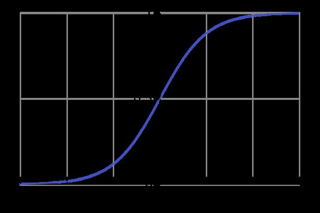
At that time, they use the logistic activation function and normal distribution initializer. They find out the variance of outputs from each layer is greater than the variance of inputs. Therefore, the output values are going to the right end or the left end. Look at the graph. The gradient of the right end or the left end is pretty saturated, it will give the answer close to zero.
当时,他们使用逻辑激活功能和正态分布初始化程序。 他们发现每层输出的方差大于输入的方差。 因此,输出值将到达右端或左端。 看一下图。 右端或左端的梯度相当饱和,它将使答案接近于零。
初始化器 (Initializer)
Our problem was the variance of the inputs is much less than the variance of the outputs. Let’s imagine you randomly drawn 10 numbers from Gaussian Distribution, the mean is 0 and the variance is 1. Then, the variance of the output will be 10. Therefore, it causes the saturation of the activation function. They suggested different initializers. It reduces the variance of the output. They consider the number of inputs and the number of neurons in layers and make the He initializer and Glorot initializer. Their variances are 1/fan(avg) and 2/fan(in). fan(avg) means the average number of inputs and neurons. fan(in) means the number of inputs. They solve the saturation problem with controlling the variance of normal distribution.
我们的问题是输入的方差远小于输出的方差。 假设您从高斯分布中随机抽取了10个数字,平均值为0,方差为1。然后,输出的方差为10。因此,它会导致激活函数饱和。 他们建议使用不同的初始化器。 它减少了输出的差异。 他们考虑输入的数量和层中神经元的数量,并制作He初始化程序和Glorot初始化程序。 它们的方差为1 / fan(avg)和2 / fan(in)。 fan(avg)表示输入和神经元的平均数量。 fan(in)表示输入数量。 他们通过控制正态分布的方差来解决饱和问题。
激活功能 (Activation Function)
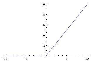
ReLU ReLUNow, we need to change the activation function because it is saturated easily at both ends. The first suggestion was the ReLU activation function. It is not saturated in the positive range. However, it was not perfect because the nodes died during training, it means the output from neurons is going to be zero. It happens especially when you set the big learning rate. The reason was the negative side always gives zero gradients.
现在,我们需要更改激活函数,因为它的两端很容易饱和。 第一个建议是ReLU激活功能。 在正范围内未饱和。 但是,这不是完美的,因为节点在训练期间死亡,这意味着神经元的输出将为零。 特别是当您设置较高的学习率时,就会发生这种情况。 原因是负边总是给出零梯度。
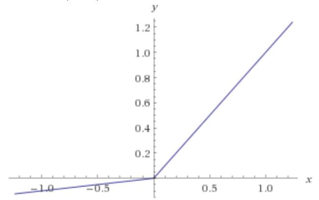
Leaky ReLU 泄漏的ReLUTo solve this problem, the Leaky ReLU is introduced. It has a positive gradient, alpha, in the negative range. The alpha can be a hyperparameter. Normally, the default value is 0.01. This value prevents the neurons from going to die.
为了解决这个问题,引入了泄漏式ReLU。 它在负范围内具有正斜率alpha。 Alpha可以是超参数。 通常,默认值为0.01。 此值可防止神经元死亡。
Note: RReLu picks the alpha randomly. PReLU learns the alpha during training, the alpha is not hyperparameter anymore.
注意:RReLu随机选择Alpha。 PReLU在训练期间学习Alpha,Alpha不再是超参数。
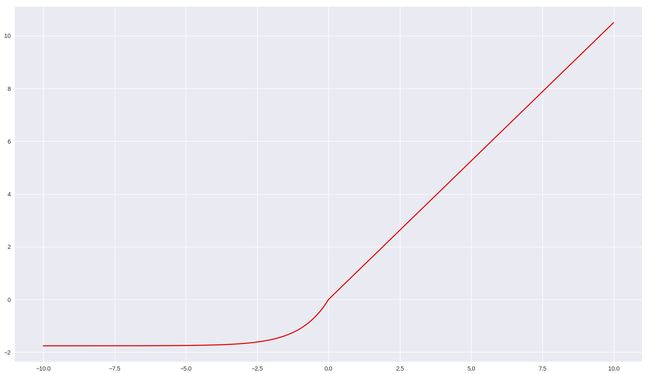
ELU ELUELU outperformed all variants of ReLU. The difference is that it uses an exponential function in the negative range, we can control the exponential function with alpha too. Therefore, it does not give the non-zero gradient. It avoids neurons dying. If alpha is 1, we can differentiate everywhere in the function.
ELU优于ReLU的所有变体。 区别在于它使用负范围内的指数函数,我们也可以使用alpha来控制指数函数。 因此,它不会给出非零梯度。 它避免了神经元死亡。 如果alpha为1,我们可以在函数中的任何地方进行区分。
SeLU SeleniumSeLU is a scaled version of ELU. Its output will be normalized, mean is 0 and variance is 1. However, there are a few conditions:
SeLU是ELU的缩放版本。 其输出将被标准化,均值为0,方差为1。但是,有一些条件:
- The input must be standardized. 输入必须标准化。
- The initializer must be the LeCun initializer. 初始化程序必须是LeCun初始化程序。
- The network must be sequential. RNN is impossible to use SeLU. 网络必须是顺序的。 RNN无法使用SeLU。
Note: The activation functions have ranked in a normal situation. SELU>ELU>leaky ReLU>ReLU>tanh>Logistice. As I mentioned, you should be careful about the conditions of SeLU.
注意:激活功能在正常情况下已排名。 SELU> ELU>泄漏的ReLU> ReLU> tanh> Logistice。 如前所述,您应该注意SeLU的条件。
批量归一化 (Batch Normalization)
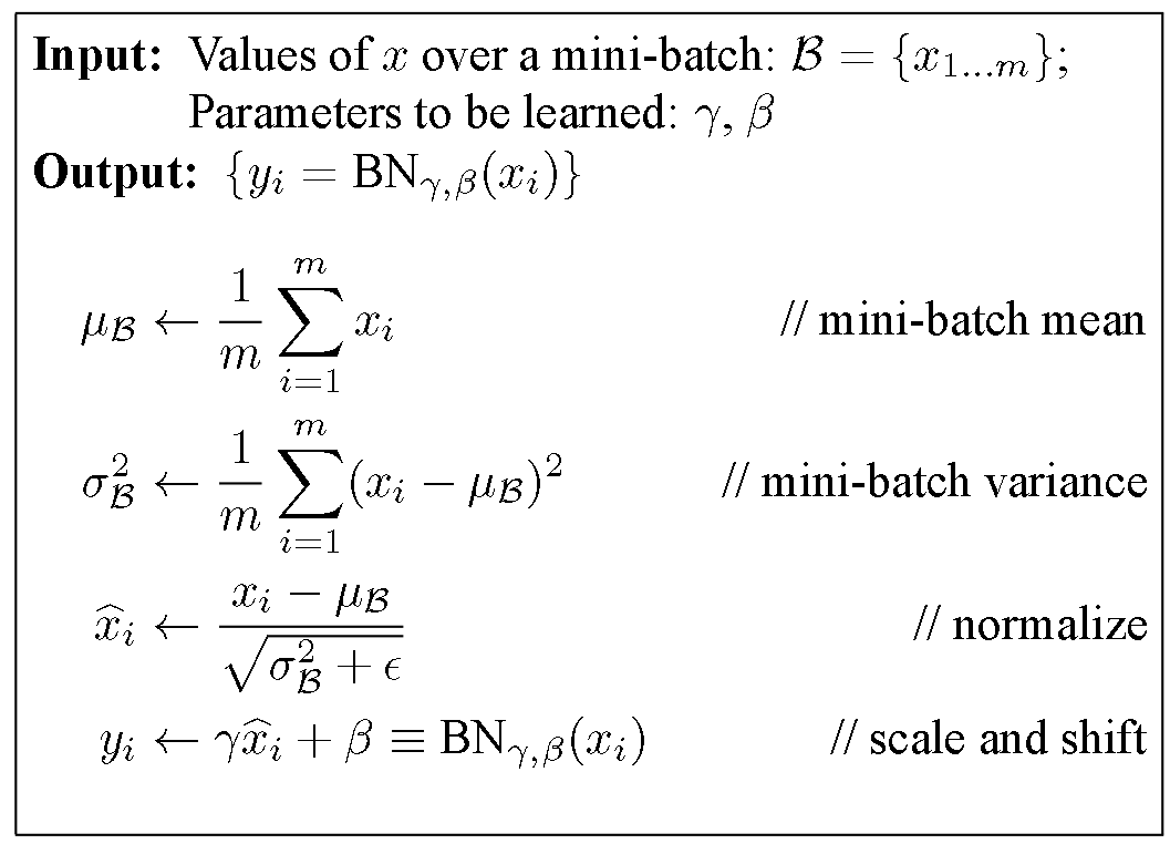
Our training speed was improved by normalized values. Then, Can we just put another algorithm to normalize the output? Yes, that is Batch Normalization. It puts the algorithm in the neuron.
归一化值提高了我们的训练速度。 然后,我们可以再放一种算法对输出进行归一化吗? 是的,那是批归一化。 它将算法放入神经元中。
This is the algorithm. We calculated the mean and the variance of the mini-batch and normalize the values. The last step is to scale it and shift it with parameters. Those 4 parameters are learned during training but the mean and the variance are only used after the training. It also acts as a regularizer. This BN layer can make training slow but convergence is faster because it goes to the optimal point with less step.
这就是算法。 我们计算了小批量的平均值和方差,并对值进行了归一化。 最后一步是对其进行缩放并使用参数对其进行移位。 这四个参数是在训练期间学习的,但均值和方差仅在训练后使用。 它还充当正则化器。 这个BN层可以使训练变慢,但是收敛更快,因为它以更少的步长到达了最佳点。
转移学习 (Transfer Learning)
Do we have to always retrain neural networks every time for a different purpose? Let’s imagine we need to build neural networks for MRI and your colleagues have the neural networks for X-ray images. Can we recycle them? Yes, we can. If you think about the structure of neural nets, you would know the output layer and the last layers have a significant role to generate the output and the output layer can be various depending on your task. Therefore, we need to change the output layer of the pre-trained model and you need to test on how deep layers you can use. You freeze whole layers, make it non-trainable, and you test your data on the pre-trained model. You can decide which layers you can use with the result.
我们是否必须总是为了不同的目的每次都重新训练神经网络? 假设我们需要建立用于MRI的神经网络,而您的同事拥有用于X射线图像的神经网络。 我们可以回收它们吗? 我们可以。 如果考虑神经网络的结构,您将知道输出层和最后一层在生成输出中起着重要作用,并且输出层可以根据您的任务而变化。 因此,我们需要更改预训练模型的输出层,并且需要测试可以使用的深度。 冻结整个图层,使其不可训练,然后在预训练的模型上测试数据。 您可以决定可以在结果中使用哪些图层。
正则化 (Regularization)
Neural Networks have massive parameters. It provides high accuracy but it causes also overfitting. Overfitting means low bias and high variance in the test data. We need to control the variance.
神经网络具有大量参数。 它提供了高精度,但也会导致过拟合。 过度拟合意味着测试数据中的低偏差和高方差。 我们需要控制方差。
l1和l2正则化 (l1 & l2 Regularization)
I explained this regularization in this post
我在这篇文章中解释了这种正则化
退出(Dropout)
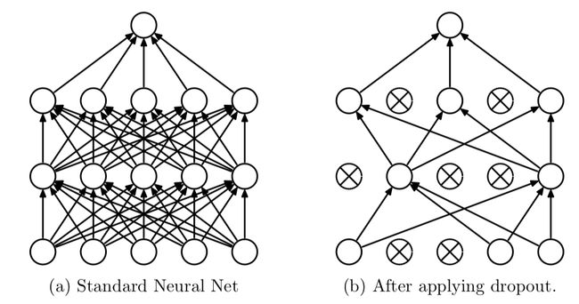
It improves your model accuracy by up to 2%. You can think this is not big but it is a lot of improvement. You will know if you stay in this field. The method is really easy. You can assign a probability to every neuron without output neurons. The probability means how likely the neurons will be un-activated in this step. The rule of thumb probability is 10~50%. RNN is 20~30%. CNN is 40%~50. It works because the neurons are trained to be tolerant of small changes. The neurons can work on different tasks because of the absence of his friends.
它将模型精度提高多达2%。 您可以认为这并不大,但是有很多改进。 您将知道是否留在此字段中。 该方法确实很简单。 您可以为没有输出神经元的每个神经元分配一个概率。 概率表示在此步骤中神经元被激活的可能性。 经验法则的概率是10〜50%。 RNN为20〜30%。 CNN为40%〜50。 之所以有效,是因为训练神经元可以容忍微小的变化。 由于没有朋友,神经元可以执行不同的任务。
蒙特卡洛辍学 (Monte Carlo Dropout)
Actually, the dropout method trains many models and use them as one model by combining their answers. However, MC Dropout pointed out this. Is it really confident about your result? It turns on the dropout and makes a prediction on the test set. It gives all different results because it is all different models. We average them and use it as the answer, it is the MC Dropout. You can get variance also.
实际上,辍学方法训练了许多模型,并通过组合其答案将它们用作一个模型。 但是,MC Dropout指出了这一点。 您对结果真的有信心吗? 它打开了辍学,并对测试集进行了预测。 因为它是所有不同的模型,所以它给出所有不同的结果。 我们将它们取平均值并将其用作答案,这是MC Dropout。 您也可以得到差异。
最大范数正则化 (Max Norm Regularization)
You can regularize the weight itself by hyperparameter and the l2 norm is used.
您可以通过超参数来规范权重本身,并使用l2范数。
优化 (Optimization)
Until now, we didn’t touch the cost function and gradient descent function. Now, we can manipulate those functions for fast training.
到目前为止,我们还没有涉及成本函数和梯度下降函数。 现在,我们可以操纵这些功能进行快速培训。
动量 (Momentum)
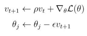
Have you ridden a bike on the hill? When you got an acceleration, you cannot stop it until you met the flat ground or you stumbled. Can we accelerate the training? Yes, we can. We don’t use the gradient as speed. We will use it as acceleration. We update momentum by the gradient. v is called momentum. rho is the fraction of momentum, it controls how much we will use the momentum. Its range is 0~1.
你在山上骑自行车了吗? 加速后,直到碰到平坦的地面或绊倒时,才能停止。 我们可以加快培训速度吗? 我们可以。 我们不使用渐变作为速度。 我们将其用作加速。 我们通过梯度更新动量。 v称为动量。 rho是动量的一部分,它控制着我们将使用多少动量。 范围是0〜1。
Nesterov加速梯度 (Nesterov Accelerated Gradient)
If you have a drone possible to watch the geographic features of the hill you are going to go down, you definitely watch it. Nesterov is doing that. As you can see, the calculation of the gradient is not on the present point. It is on the estimated future point. It makes faster training than momentum in almost all cases.
如果您有无人机可以观看要下山的地理特征,那么您肯定会观看。 内斯特罗夫正在这样做。 如您所见,梯度的计算不在当前点上。 它在估计的未来点上。 在几乎所有情况下,它都比动量训练更快。
阿达格拉德 (AdaGrad)
We can change the learning rate during training. It does not use in Neural Net anymore but it influences a lot of methods. Other methods bounce a lot. They are also too fast to stop at global minima. It is designed to slow down the speed near the global optima. They store momentum and divide the learning rate. Therefore, the speed will go down during the training. Its major problem is slowing down a bit too fast.
我们可以在培训期间更改学习率。 它不再在神经网络中使用,但会影响许多方法。 其他方法反弹很多。 他们也太快了,不能停在全球最低水平。 它旨在减慢接近全局最优值的速度。 他们储存动力并划分学习率。 因此,在训练过程中速度会下降。 它的主要问题是放慢速度太快。
Note: RMSprop solved this problem by storing a small portion of momentum.
注意: RMSprop通过存储一小部分动量来解决此问题。
亚当和纳丹 (Adam & Nadam)
Adam is a combination of AdaGrad and Momentum. Nadam is adam with Nesterov Accelerated Gradient.
亚当是AdaGrad和Momentum的组合。 纳达姆(Nadam)与Nesterov Accelerated Gradient一起使用亚当。
If you need more explanation or more optimizer, you can check this: https://ruder.io/optimizing-gradient-descent/index.html#nadam
如果您需要更多说明或更多优化器,则可以进行以下检查: https : //ruder.io/optimizing-gradient-descent/index.html#nadam
This post is published on 9/27/2020
此帖发布于9/27/2020
翻译自: https://medium.com/swlh/basics-of-deep-learning-2d2407d371fd
深度学习 机器学习基础


