3D点云重建0-06：MVSNet-源码解析（2）-网络框架结构总览

以下链接是个人关于MVSNet(R-MVSNet)-多视角立体深度推导重建 所有见解，如有错误欢迎大家指出，我会第一时间纠正。有兴趣的朋友可以加微信：17575010159 相互讨论技术。若是帮助到了你什么，一定要记得点赞！因为这是对我最大的鼓励。$文末附带$$公众号-$$海量资源。$

3D点云重建0-00：MVSNet(R-MVSNet)–目录-史上最新无死角讲解：https://blog.csdn.net/weixin_43013761/article/details/102852209

代码详细注解

大家先把下面的代码直接过一遍，不要去琢磨细节（后面我会带大家详细的去分析没一个要点）mvsnet/train.py：

def train(traning_list):
	......
	#  数据预处理部分
	......
        for i in range(FLAGS.num_gpus):
            with tf.device('/cpu:%d' % i):
                with tf.name_scope('Model_tower%d' % i) as scope:
                    # generate data
                    # 获得训练一次，所需要的训练样本，包含图片像素，摄像头参数，以及对应的深度图
                    images, cams, depth_image = training_iterator.get_next()
                    # 重新改变输入像素的形状，其包含了r img以及s img
                    images.set_shape(tf.TensorShape([None, FLAGS.view_num, None, None, 3]))
                    # 改变摄像头参数的形状，其包含了extrinsic以及intrinsic信息
                    cams.set_shape(tf.TensorShape([None, FLAGS.view_num, 2, 4, 4]))
                    depth_image.set_shape(tf.TensorShape([None, None, None, 1]))

                    # 这里获的摄像头参数对，并且切割出深度开始的数值，以及深度的间隔（可以理解理解为）
                    depth_start = tf.reshape(
                        tf.slice(cams, [0, 0, 1, 3, 0], [FLAGS.batch_size, 1, 1, 1, 1]), [FLAGS.batch_size])
                    depth_interval = tf.reshape(
                        tf.slice(cams, [0, 0, 1, 3, 1], [FLAGS.batch_size, 1, 1, 1, 1]), [FLAGS.batch_size])

                    is_master_gpu = False
                    if i == 0:
                        is_master_gpu = True

                    # inference
                    # 如果为MVSNet模型
                    if FLAGS.regularization == '3DCNNs':

                        # initial depth map，构建深度图推导的网络
                        with tf.device('gpu:%d' % i):
                            # 这里会返回一个推导出来的深度图，以及一个概率分布图
                            depth_map, prob_map = inference(
                                images, cams, FLAGS.max_d, depth_start, depth_interval, is_master_gpu)

                        # refinement，对深度图进行提炼，理解为质量加强即可
                        if FLAGS.refinement:
                            # 获得r img
                            ref_image = tf.squeeze(
                                tf.slice(images, [0, 0, 0, 0, 0], [-1, 1, -1, -1, 3]), axis=1)
                            # 通过r img与推断的到depth_map的结合，获得精炼的特征图
                            refined_depth_map = depth_refine(depth_map, ref_image,
                                    FLAGS.max_d, depth_start, depth_interval, is_master_gpu)
                        else:
                            refined_depth_map = depth_map

                        # regression loss，接下来为重点，涉及到loss部分
                        # depth_image为标签的深度图，depth_map为网络推断出来的深度图，depth_interval为深度最小单位间隔
                        # 可以看到，求了两次loss，一次是与提炼的深度图，一次是和没有提炼的深度图
                        loss0, less_one_temp, less_three_temp = mvsnet_regression_loss(
                            depth_map, depth_image, depth_interval)
                        loss1, less_one_accuracy, less_three_accuracy = mvsnet_regression_loss(
                            refined_depth_map, depth_image, depth_interval)
                        # 两次loss去平均值
                        loss = (loss0 + loss1) / 2

                    elif FLAGS.regularization == 'GRU':

                        # probability volume
                        prob_volume = inference_prob_recurrent(
                            images, cams, FLAGS.max_d, depth_start, depth_interval, is_master_gpu)

                        # classification loss
                        loss, mae, less_one_accuracy, less_three_accuracy, depth_map = \
                            mvsnet_classification_loss(
                                prob_volume, depth_image, FLAGS.max_d, depth_start, depth_interval)

                    # retain the summaries from the final tower.
                    summaries = tf.get_collection(tf.GraphKeys.SUMMARIES, scope)

                    # calculate the gradients for the batch of data on this CIFAR tower.
                    # 计算梯度，并且进行优化
                    grads = opt.compute_gradients(loss)

                    # keep track of the gradients across all towers.
                    tower_grads.append(grads)
        
        # average gradient，计算平均的梯度
        grads = average_gradients(tower_grads)
        
        # training opt
        train_opt = opt.apply_gradients(grads, global_step=global_step)
		......

框架解析

其实呢，上面的核心代码就下面几处：

depth_map, prob_map = inference(
    images, cams, FLAGS.max_d, depth_start, depth_interval, is_master_gpu)

对应论文中的下面部分：

还有就是

refined_depth_map = depth_refine(depth_map, ref_image,
        FLAGS.max_d, depth_start, depth_interval, is_master_gpu)

对应论文中如下部分：

然后就是

     # regression loss，接下来为重点，涉及到loss部分
     # depth_image为标签的深度图，depth_map为网络推断出来的深度图，depth_interval为深度最小单位间隔
     # 可以看到，求了两次loss，一次是与提炼的深度图，一次是和没有提炼的深度图
     loss0, less_one_temp, less_three_temp = mvsnet_regression_loss(
         depth_map, depth_image, depth_interval)
     loss1, less_one_accuracy, less_three_accuracy = mvsnet_regression_loss(
         refined_depth_map, depth_image, depth_interval)

也就是网络loss的构建。接下来的博客，我会对这3个部分进行详细的讲解。

inference

首先我们来看看其中的：

	# 这里会返回一个推导出来的深度图，以及一个概率分布图
	depth_map, prob_map = inference(
	    images, cams, FLAGS.max_d, depth_start, depth_interval, is_master_gpu)

其代码的实现在mvsnet/model.py中，还是一样，大家先总体的浏览一下，不要去纠结一些细节，针对细节我后面有详细的讲解：

def inference(images, cams, depth_num, depth_start, depth_interval, is_master_gpu=True):
    """
    infer depth image from multi-view images and cameras ,根据多个视角图（s img），推断出r img的深度图
    :param images: images[0]表示的是s img，其余的都表示r img
    :param cams: 摄像头的参数，与摄像头是一一对应的
    :param depth_num: 深度的最大上限，可以理解为又多少个depth_interval
    :param depth_start: 起始深度
    :param depth_interval: 深度间隔
    :param is_master_gpu: 是否为主GPU
    :return:
    """


    # dynamic gpu params，根据depth_num，以及depth_start计算出最大深度值
    depth_end = depth_start + (tf.cast(depth_num, tf.float32) - 1) * depth_interval

    # reference image，切割出r img以及拍摄该图片时，摄像头的参数
    ref_image = tf.squeeze(tf.slice(images, [0, 0, 0, 0, 0], [-1, 1, -1, -1, 3]), axis=1)
    ref_cam = tf.squeeze(tf.slice(cams, [0, 0, 0, 0, 0], [-1, 1, 2, 4, 4]), axis=1)

    # image feature extraction，对r img进行2D特征提取，该处只是获得了UNetDS2GN的类对象而已，没有对网络进行构建
    # 如果是master_gpu，说说明第一册构建UNetDS2GN，此时不重复使用权重，否则使用和主GPU相同的权重
    if is_master_gpu:
        ref_tower = UNetDS2GN({'data': ref_image}, is_training=True, reuse=False)
    else:
        ref_tower = UNetDS2GN({'data': ref_image}, is_training=True, reuse=True)


    # 为每个视觉图的推导，创建一个UNetDS2GN对象，其权重和第一层创建UNetDS2GN的权重相同
    view_towers = []
    for view in range(1, FLAGS.view_num):
        view_image = tf.squeeze(tf.slice(images, [0, view, 0, 0, 0], [-1, 1, -1, -1, -1]), axis=1)
        view_tower = UNetDS2GN({'data': view_image}, is_training=True, reuse=True)
        view_towers.append(view_tower)

    # get all homographies，获得每个视觉（r img以及s img）的homographies
    view_homographies = []
    for view in range(1, FLAGS.view_num):
        # 获得视觉图对应的摄像头配置参数
        view_cam = tf.squeeze(tf.slice(cams, [0, view, 0, 0, 0], [-1, 1, 2, 4, 4]), axis=1)

        # 传入r img摄像头参数以及s img的摄像头参数，得到homographies,注意这里每次都是ref_cam与一个view_cam传入
        # ref_cam[batch_size,2,4,4], view_cam[batch_size,2,4,4]，homographies(?, 192, 3, 3)
        homographies = get_homographies(ref_cam, view_cam, depth_num=depth_num,
                                        depth_start=depth_start, depth_interval=depth_interval)

        view_homographies.append(homographies)

    # build cost volume by differentialble homography
    with tf.name_scope('cost_volume_homography'):
        depth_costs = []
        # 对每个深度都进行计算
        for d in range(depth_num):
            # compute cost (variation metric)
            ave_feature = ref_tower.get_output()
            # 对每个求平方
            ave_feature2 = tf.square(ref_tower.get_output())
            for view in range(0, FLAGS.view_num - 1):
                # 获得对应的深度的homography[b,3,3],并且进行平方计算
                homography = tf.slice(view_homographies[view], begin=[0, d, 0, 0], size=[-1, 1, 3, 3])
                homography = tf.squeeze(homography, axis=1)

                # warped_view_feature = homography_warping(view_towers[view].get_output(), homography)
                #传入对应视觉图抽取出来的特征向量，以及转化到r img的homography参数，
                #这里，可以这样认为，把s img视觉的的特征，通过单应性转换到r img特征去
                warped_view_feature = tf_transform_homography(view_towers[view].get_output(), homography)
                ave_feature = ave_feature + warped_view_feature
                ave_feature2 = ave_feature2 + tf.square(warped_view_feature)

            # 然后所有视觉图（r img以及 s img）得特征图求平均值，
            ave_feature = ave_feature / FLAGS.view_num
            ave_feature2 = ave_feature2 / FLAGS.view_num

            # 假设，如果s img的特征向量映射到r img特征向量是完美映射，也就是两个完全相同（当然，这是不可能的），则cost等于0
            # 如果cost不为0，则表示他们存在视角差，单次是计算一个深度的视觉差
            cost = ave_feature2 - tf.square(ave_feature)

            depth_costs.append(cost)

        # 该处集合了各个深度的视觉差,我们就是根据这些视觉差，或者说3D损耗去进行深度图的推导
        cost_volume = tf.stack(depth_costs, axis=1)

    # filtered cost volume, size of (B, D, H, W, 1)=(?, 192, ?, ?, 1)
    # 这里完成的是论文图示的Cost Volume Regularization操作，带有反卷积操作，对初始的cost_volume进行过滤
    if is_master_gpu:
        filtered_cost_volume_tower = RegNetUS0({'data': cost_volume}, is_training=True, reuse=False)
    else:
        filtered_cost_volume_tower = RegNetUS0({'data': cost_volume}, is_training=True, reuse=True)

    # 进行维度压缩得到[B, D, H, W]
    filtered_cost_volume = tf.squeeze(filtered_cost_volume_tower.get_output(), axis=-1)

    # depth map by softArgmin
    with tf.name_scope('soft_arg_min'):
        # probability volume by soft max
        # tf.scalar_mul为标量与矢量相乘，这里乘以-1，等于加上了-号，
        # 对3D立体的volume每个立体像素，都进行深度预测
        # probability_volume[B, D, H, W],
        probability_volume = tf.nn.softmax(
            tf.scalar_mul(-1, filtered_cost_volume), axis=1, name='prob_volume')


        # depth image by soft argmin
        # 获得probability_volume的形状[B, D, H, W]
        volume_shape = tf.shape(probability_volume)
        soft_2d = []
        # 对每个样本进行处理
        for i in range(FLAGS.batch_size):
            # 对每个样本，根据depth_start[i], depth_end[i]的不同，但是划分成depth_num份
            # tf.linspace使用，如tf.linspace(0,5,5)=[0,1,2,3,4]
            soft_1d = tf.linspace(depth_start[i], depth_end[i], tf.cast(depth_num, tf.int32))
            soft_2d.append(soft_1d)
        # [b,d,1,1]
        soft_2d = tf.reshape(tf.stack(soft_2d, axis=0), [volume_shape[0], volume_shape[1], 1, 1])
        # [b,d,h,w]
        soft_4d = tf.tile(soft_2d, [1, 1, volume_shape[2], volume_shape[3]])

        #estimated_depth_map[b,h,w], 这个地方注意以下，probability_volume在前面是乘以了-1，
        # 我们把soft_4d想成一个立体空间，假设其中放了一个物体，那么这个物体在这个空间肯定占据了很多立体像素
        # 把d这个维度的像素都加起来，这个值越大就代表物体的占用越深，那么离表面就越近。
        # 但是相加的时候乘以了个probability_volume，其为负数，则反过来，改值越大，则离开表面越远，这样就形成了深度图
        estimated_depth_map = tf.reduce_sum(soft_4d * probability_volume, axis=1)
        # [b,h,w,1]
        estimated_depth_map = tf.expand_dims(estimated_depth_map, axis=3)

    # 获得深度概率分布图
    prob_map = get_propability_map(probability_volume, estimated_depth_map, depth_start, depth_interval)
    return estimated_depth_map, prob_map#, filtered_depth_map, probability_volume

其上的代码，核定点有如下几个：

	ref_tower = UNetDS2GN({'data': ref_image}, is_training=True, reuse=False)
	for view in range(1, FLAGS.view_num):
        homographies = get_homographies(ref_cam, view_cam, depth_num=depth_num,depth_start=depth_start,depth_interval=depth_interval)

这里就是为了提取r img以及s img的特征图，也就是论文中如下图示部分：

在接下来就是：

with tf.name_scope('cost_volume_homography'):
	.......
	.......
	cost_volume = tf.stack(depth_costs, axis=1)

这部分代码了，对应论文中如下部分：

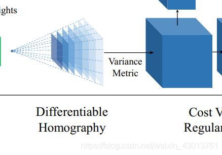
其中cost_volume就是表示上面的立方体。

在接下来就是

	filtered_cost_volume_tower = RegNetUS0({'data': cost_volume}, is_training=True, reuse=False)

对上面生成的cost_volume进行滤波操作，也就是论文中的这个部分：

最后就是：

    # depth map by softArgmin
    with tf.name_scope('soft_arg_min'):
    	......
    	......
    return estimated_depth_map, prob_map#, filtered_depth_map, probability_volume

也就是论文中的：

这样我们就一一对应起来了，但是对于每个环节的细节，我们还不是很了解，这些就是我们后面要去分析的内容了。