K-means and K-means++
Kmenas
K-means is the simplest implementation of the maximum separation and maximum cohesion principles. Suppose we have a dataset![]() (being M N-dimensional samples). And it shall be divided into K clusters and a group of K centroids corresponding to the sample mean assigned to each cluster
(being M N-dimensional samples). And it shall be divided into K clusters and a group of K centroids corresponding to the sample mean assigned to each cluster![]() .
.
![]()
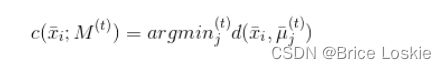
集合M和质心有一个附加索引(作为上标)指示迭代步骤。从最初的猜测![]() 开始,K-means试图最小化称为惯性的目标函数(即分配给聚类Kj的样本与其质心μj之间的总平均聚类内距离):
开始,K-means试图最小化称为惯性的目标函数(即分配给聚类Kj的样本与其质心μj之间的总平均聚类内距离):
很容易理解不能将S(t)视为绝对度量,因为其值受样本方差的影响很大。然而S(t+1)
完成所有分配后,新的质心将重新计算作为算术平均值:

重复该过程直到质心停止变化(这也意味着序列S(0)>S(1)>…> S(![]() ))。读者应该能立刻理解最初的猜测对计算时间有很大的影响。如M(0)非常接近
))。读者应该能立刻理解最初的猜测对计算时间有很大的影响。如M(0)非常接近![]() 通过几次迭代即可找到最佳配置。相反,当M(0)纯粹是随机的时候,无效的初始选择的概率接近1(也就是说,每个初始的统一随机选择在计算复杂性方面几乎是等价的。
通过几次迭代即可找到最佳配置。相反,当M(0)纯粹是随机的时候,无效的初始选择的概率接近1(也就是说,每个初始的统一随机选择在计算复杂性方面几乎是等价的。
K-means++
找到最佳初始配置相当于最小化惯性;然而,Arthur和Vassilvitskii(在K-means++: The Advantages of Careful Seeding和Proceedings of the Eighteenth Annual ACM-SIAM Symposium on Discrete Algorithms中)提出了另一种初始化方法(称为K-means++),该方法通过选择有更高概率接近最终质心的初始质心,从而显著提高了收敛速度。该方法完整的证明是相当复杂的,可以在上述的参考资料中找到。因此,我们直接提供最终结果和一些重要的成果。
让我们来考虑函数D(•),其被定义为:
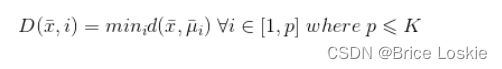
D(•)表示样本x∈X与已经选定的质心之间的最短距离。计算函数后,就可以确定概率分布G(x):

第一质心 是从均匀分布中取样。此时,可以为所有x∈X的样本计算D(•),因此可以计算概率分布G(x)。很坦率地说,如果我们从G(x)中采样,在稠密区域中选择一个值的概率远大于均匀采样或在分离区域中选择质心的概率。因此,我们继续从G(x)中采样μ2。重复该过程直到确定所有的K质心。当然,由于这是一种概率方法,我们无法保证最终配置是最优的。然而,K-means++是具有O(log K)竞争性的。事实上,如果Sopt是S在理论上的最佳值,作者证明了以下不等式是成立的:事实上,如果Sopt是S在理论上的最佳值,作者证明了以下不等式是成立的:

当S由于更好的选择而减少时,前面的公式将为预期值E[S]设置一个上限,大致与log K成正比。例如对于K=10,E[S][插图]19.88 • Sopt;而对于K=3,E[S][插图]12.87 • Sopt。这一结果揭示了两点:第一点是K-means++在K不是非常大时表现更好;第二个点可能也是最重要的点,就是单个K-means++初始化不足以获得最佳配置。因此,常见的实现(例如scikit-learn)是执行可变数量的初始化,并选择初始惯性最小的初始化。
K-means++ 实现
K-means算法的一个缺点是它对质心或平均点的初始化敏感。因此,如果一个质心被初始化为一个“遥远”的点,它可能最终没有与之关联的点,同时,多个簇可能最终与单个质心链接。类似地,可能会将多个质心初始化到同一个簇中,从而导致较差的聚类。例如,考虑下面显示的图像。质心初始化不好导致聚类不好。
# importing dependencies
import numpy as np
import pandas as pd
import matplotlib.pyplot as plt


# creating data
mean_01 = np.array([0.0, 0.0])
cov_01 = np.array([[1, 0.3], [0.3, 1]])
dist_01 = np.random.multivariate_normal(mean_01, cov_01, 100)

mean_02 = np.array([6.0, 7.0])
cov_02 = np.array([[1.5, 0.3], [0.3, 1]])
dist_02 = np.random.multivariate_normal(mean_02, cov_02, 100)

mean_03 = np.array([7.0, -5.0])
cov_03 = np.array([[1.2, 0.5], [0.5, 1,3]])
dist_03 = np.random.multivariate_normal(mean_03, cov_01, 100)

mean_04 = np.array([2.0, -7.0])
cov_04 = np.array([[1.2, 0.5], [0.5, 1,3]])
dist_04 = np.random.multivariate_normal(mean_04, cov_01, 100)

data = np.vstack((dist_01, dist_02, dist_03, dist_04))
np.random.shuffle(data)

# function to plot the selected centroids
def plot(data, centroids):
	plt.scatter(data[:, 0], data[:, 1], marker = '.',
				color = 'gray', label = 'data points')
	plt.scatter(centroids[:-1, 0], centroids[:-1, 1],
				color = 'black', label = 'previously selected centroids')
	plt.scatter(centroids[-1, 0], centroids[-1, 1],
				color = 'red', label = 'next centroid')
	plt.title('Select % d th centroid'%(centroids.shape[0]))

	plt.legend()
	plt.xlim(-5, 12)
	plt.ylim(-10, 15)
	plt.show()

# function to compute euclidean distance
def distance(p1, p2):
	return np.sum((p1 - p2)**2)

# initialization algorithm
def initialize(data, k):
	'''
	initialized the centroids for K-means++
	inputs:
		data - numpy array of data points having shape (200, 2)
		k - number of clusters
	'''
	## initialize the centroids list and add
	## a randomly selected data point to the list
	centroids = []
	centroids.append(data[np.random.randint(
			data.shape[0]), :])
	plot(data, np.array(centroids))

	## compute remaining k - 1 centroids
	for c_id in range(k - 1):

		## initialize a list to store distances of data
		## points from nearest centroid
		dist = []
		for i in range(data.shape[0]):
			point = data[i, :]
			d = sys.maxsize

			## compute distance of 'point' from each of the previously
			## selected centroid and store the minimum distance
			for j in range(len(centroids)):
				temp_dist = distance(point, centroids[j])
				d = min(d, temp_dist)
			dist.append(d)

		## select data point with maximum distance as our next centroid
		dist = np.array(dist)
		next_centroid = data[np.argmax(dist), :]
		centroids.append(next_centroid)
		dist = []
		plot(data, np.array(centroids))
	return centroids

# call the initialize function to get the centroids
centroids = initialize(data, k = 4)