【ISE3002: Planning of Production and Service Systems】(TBC)
Planning of Production and Service Systems Learning Notes
Content derived from The Hong Kong Polytechnic University ISE3002 courses
Content
- Chapter 1: The Systems Concept
-
- The Transformational Model of a System
-
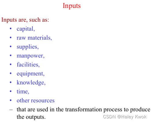
- Input
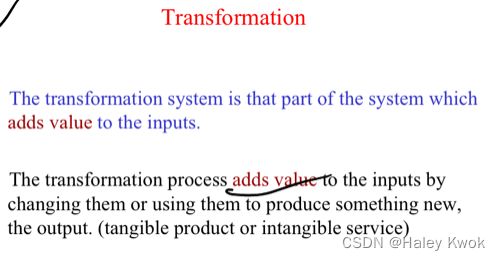
- Transformation
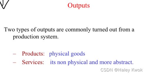
- Outputs
- Environment
- Example
- Chapter 2: Capacity Planning
-
- 1. Design Capacity
- 2. Effective Capacity
-
- Example
- 3. Strategies for Modifying Capacity
-
- Expansion
- Contraction and Constant Capacity
- Chapter 3: Forecasting
-
-
- Elements of a Good Forecast
- External
- Internal
- Approaches to Forecasting
-
- Qualitative Forecasting Techniques
- Quantitative Forecasting Techniques (Forecasting Models):
-
- 1) Time Series Model
- Seasonal Fluctuation (Seasonality)
- Cyclical Variation
- Irregular variations
- Residual Unexplained Variations
-
- 1) Moving Average:
- Characteristics
- 2) Weighted moving average
- 3) Exponential Smoothing
-
- Choice of alpha value
- Mean Absolute Deviation (MAD)
- Bias
- **Least Mean Squares Method
- Determination of the Seasonal Component
-
- Multiplicative Seasonal Method
-
- Example: The “Quarterly Average Method”
- Example: The “Ratio to Trend Method”
- 2) Causal Model
-
- Simple Linear Regression
- Multiple Linear Regression
- 3) Econometric models
-
- Forecast Accuracy and Control
- Correlation analysis
-
- Coefficient of determination ( R)
- Coefficient of correlation ( r)
- MAD: Forecast Control using "Tracking Signal" method
-
- Chapter 4: Aggregate Planning 总体规划
-
- Aggregate Planning V.S. Capacity Planning
-
- 1. Levels of Capacity Planning
- 2. Relationship of Scheduling Activities
- 3. The Concept of Aggregation
-
- Master Scheduling (Disaggregation)
- Master Production Schedule (MPS)
- Material Requirement Planning (MRP)
- Loading
- Sequencing
- Scheduling
- Dispatching
- 4. Aggregate Production Planning
-
- 4.1 A pure strategy
-
- Examples
- Modify capacity
- Modify output
- Steps in Aggregate Planning
-
- 4.2 Planning Strategy
- 4.3 Chase strategies
- 4.4 Level Strategies
- 4.5 A mixed strategy
- Example 1
- Strategy 1: Chase Strategy
- Strategy 2: Level Strategy
- Strategy 3:
- Strategy 4:
- Example 2
- Methods of Aggregate Planning
-
- Example 1 (PPSS):
- Example 2
- Chapter 5: Master Production Planning – Master Production Schedule (MPS)
-
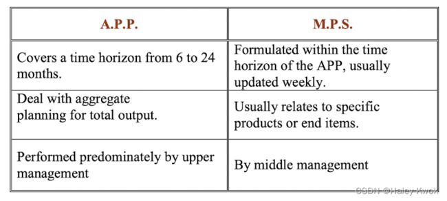
- Aggregate Planning V.S. Master Scheduling
- Capacity and Priority Planning
-
- Priority planning
- Capacity planning
- Capacity Requirement Planning (CRP)
- Time Cycle Chart
- Master Schedule Revision
- Chapter 6: Inventory Management and Control
-
- Principle Kinds of Stocks
-
- Stock costs
- 1. A typical inventory control system
- 2. Stock Control Systems
-
- 1) The fixed reorder quantity system
-
- a) The maximum and minimum ordering system
- a) The maximum and minimum ordering system (with safety stock)
- b) Perpetual Inventory System
- 2) The order cycle system (the fixed reorder interval system)
-
- Optional Replenishment Inventory System (with reorder point)
- 3. Material Requirement Planning (MRP)
- 4. Economic Order/Batch Size (EOQ)
-
- A) For Raw Materials, WIP and Final Inventory
- B) For Purchased Items:
- 5. Economic Order/Batch Quantity
-
- Model I
-
- Find the optimum batch size q o p t q_{opt} qopt
- The Economic Reorder Point ( R)
- Quantity Discounts
- Model II
- 6. Pareto Analysis (ABC classification) of stock items
-
- Pareto Analysis
- ABC Classification
- ABC (Pareto) Analysis
- Selective inventory control
- Advantages
- Chapter 7: Material Requirements Planning (MRP)
-
- The major objectives of an MRP system are to:
- Key features of an MRP system
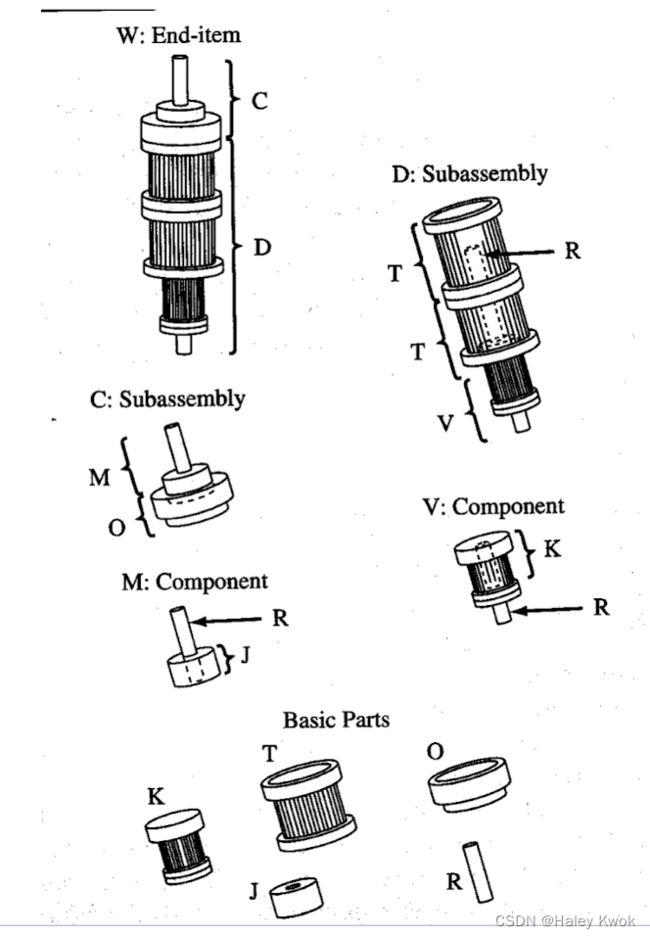
- 1. Product Structure
-
- 1.1 Independent demand
- 1.2 Dependent demand
- 2. MRP Inputs
- 3. MRP Outputs
- 4. The Material Requirement Planning (MRP) Process
- 5. MRP Computation
-
- IMPORTANT COMPONENTS
- The MRP
- Lot sizing
-
- Period order quantity (POQ) Method
- Part-Period Balancing Method
- The Economic Part Period Method (EPP)
- ERP
- Exercise
- Chapter 8: Operations Loading and Scheduling
-
- 1. Loading
-
- Bar Chart
- The Gantt (Load) Chart
- Index Method (For Loading Jobs to Machines)
- 2. Scheduling
-
- Master Scheduling
- Detailed Scheduling
- Approaches
- A Gantt (Scheduling) Chart
- 3. Sequencing
-
- Johnson's Algorithm (Sequence jobs for 2 machines)
- Sequence jobs for 3 machines
- Cambell, Dudek and Smith Algorithm (C-D-S Algorithm, for sequencing N jobs to M machines)
- Critical Ratio (for reference)
-
- Priority Rules
- Chapter 9: Just-in-Time (JIT)/ Lean Manufacture
-
- 1. Main Elements of JIT/Lean Production
- 2. Inventory Hides Problems
- 3. Wastages
-
- Categories of Waste
- 4. Man-hour reduction
-
- 4.1 Elimination of waste
- 4.2 Redistribution of works
- 5. JIT Layout
- 6. Leveling (Smoothing out) the Production System
-
- Load smoothing in quantities and types
- 7. Reduction of Machine Set-up Time
-
- An Approach for Set-up time Reduction
-
- 1) Separating the internal set-up from the external set-up activities.
- 2) Further reducing internal set-up by
- 8. Shorten the Lead time
- 9. Reduce Inventory
- 10. Zero Inventory as A Challenge
- 11. The "Kanban" System
-
- Two basic types of kanbans
- Advantages of Kanban
- Determining the number of Kanbans
- 12. JIT Partnership
- 13. Quality Circles
- 14. Implementation of JIT
Chapter 1: The Systems Concept
The Transformational Model of a System

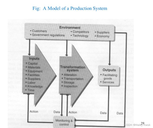
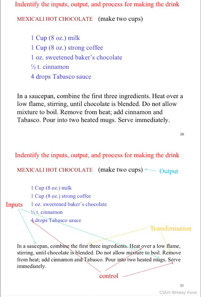
Input
Transformation

Outputs
Environment

Example
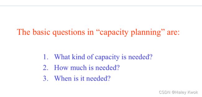
Chapter 2: Capacity Planning
Capacity of a facility: the maximum rate of production or service capability of a company’s operation.
Usually expressed as L volume of output per time period. (e.g., units/week, customers/hr et.)

1. Design Capacity
The maximum output that can possibly be attained per unit time.
2. Effective Capacity
The maximum possible output attainable per unit time given
– a product mix,
– scheduling difficulties,
– m/c maintenance,
– quality factor, etc
Actual output: The output per unit time actually achieved.
Efficiency = Actual output / Effective capacity
Utilization = Actual output / Design capacity
Example

3. Strategies for Modifying Capacity


Product = Sale Revenue - Cost (fixed + variable)
Expansion
If demand is anticipated to be permanently higher, facilities should be expanded to heap the benefits of economics of scale offered by a larger facility.


Contraction and Constant Capacity
Selling off existing facilities, equipment and inventory; firing employees (last resort).
Seeking new ways to maintain and use existing capacity.
Chapter 3: Forecasting
Demand Forecast:
– The estimation of the future trend and expectation of
the demand of a business based on analysis of past data, or on judgement and opinion
e.g., long range/ medium range/ short range demand forecast
Elements of a Good Forecast
Timely: the forecasting horizon must cover the time necessary to implement possible changes.
Accurate: the degree of accuracy (possible error) should be stated. Reliable: a forecast technique should work consistently.
Simple and easy: forecasts should be made in simple and written forms that can be easily understood and used.
Cost effective: the benefit should outweigh the costs.
External
Available statistics: e.g.
– The national Economic Health Pricing Index,
– Consumers - spending trends,
– Trading, import and export figures, etc
Internal
Data specific to the products of the company, eg:
- Historical Data (sales records, customer orders, production orders….)
- Opinions:
Consumer Opinion, Customer Opinion, Executive Opinion - Market Research
- Marketing Trials
- Distributor Survey
Approaches to Forecasting
Forecasting Procedure:
The basis steps are:
- Identify the product or service (group) for demand forecast.
- Determine the purpose of the forecast.
- Establish a time horizon.
- Select a forecasting technique.
- Collect, clean and analyze appropriate data.
- Make the forecast.
- Monitor the forecast.
Qualitative: Forecast based on subjective inputs. (Delphi Method, Expert judgement, executive opinions, sales force opinions, consumer surveys.)
Quantitative: Forecast based on analysis of historical data or causal variables. (Time series models, trend projection methods, regression analysis)
Qualitative Forecasting Techniques
- Consumer Survey: The opinions of consumers are surveyed and analysed to
produce the forecast. - Sales Force Composite Method: Opinions of sales and marketing people are taken and analysed to produce the forecast.
- Jury of Executives Opinion: Opinions of executives are taken and analysed to produce the forecast.
The Delphi Technique:
- In this method, a attempt is made to develop forecasts through “group consensus” by the knowledgeable people/experts.
- Series of questionnaires are answered anonymously by members of the panel.
- The goal is to produce a relatively narrow spread of opinions within which the majority of the members concur.
- Generally used for long range forecasts. (Others, eg., regarding scientific advances, changes in society, government regulations, and the competitive environment, etc )
Quantitative Forecasting Techniques (Forecasting Models):
Broadly speaking,
– 2 basic types of techniques:
1) Time Series Model
Here, the variables to be forecasted is analysed historically over time and the pattern or patterns are modelled and estimated.
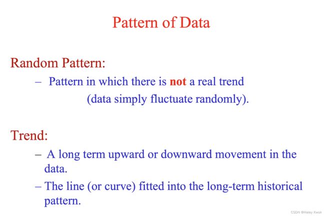
Seasonal Fluctuation (Seasonality)
Pattern in which fluctuations in the data
– occur during some fixed time period of one year or less according to some seasonal factor,
– repeats itself over each consecutive time period.
Cyclical Variation
Pattern which is similar to the seasonal pattern, except that
– the time period is not one year and
– the cycles do not necessarily form a repeating pattern.
– the magnitude, timing and pattern of cyclic fluctuation vary so widely and are due to so many causes.
– generally impractical to forecast them.
Irregular variations
– Variations due to unusual circumstances.
– Their inclusion can distort the overall picture and should be identified and removed from the data.
Residual Unexplained Variations
– The elements which can not be forecasted.
e.g. “Acts of God”, sudden change in politics.

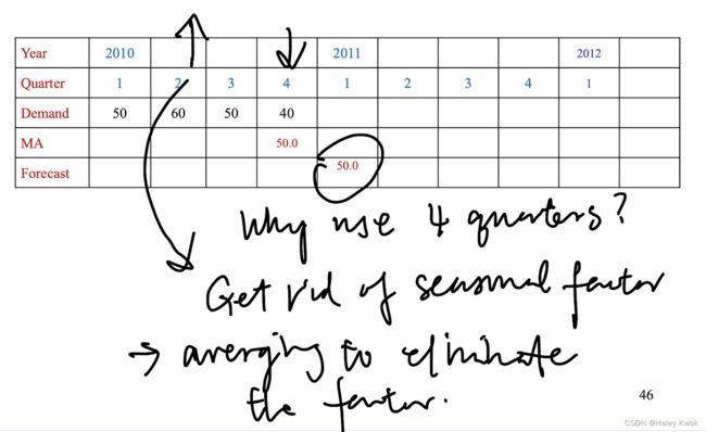
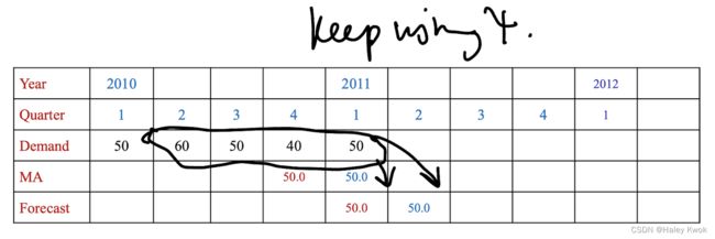
1) Moving Average:
A moving average forecast is obtained by summing and averaging the data points over a desired number of past periods (N).
– This number usually encompasses a seasonal cycle in order to smooth out seasonal variations.
Characteristics
– The method is not influenced by very old data
– The method does not reflect solely the figure for the previous period.
– It smoothes the pattern of figures.
– It indicates the trend of the figures

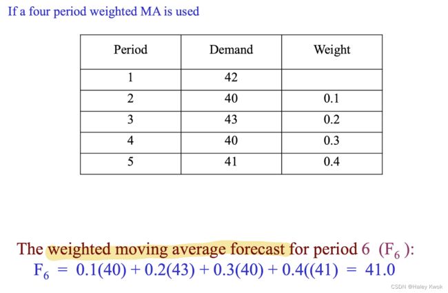
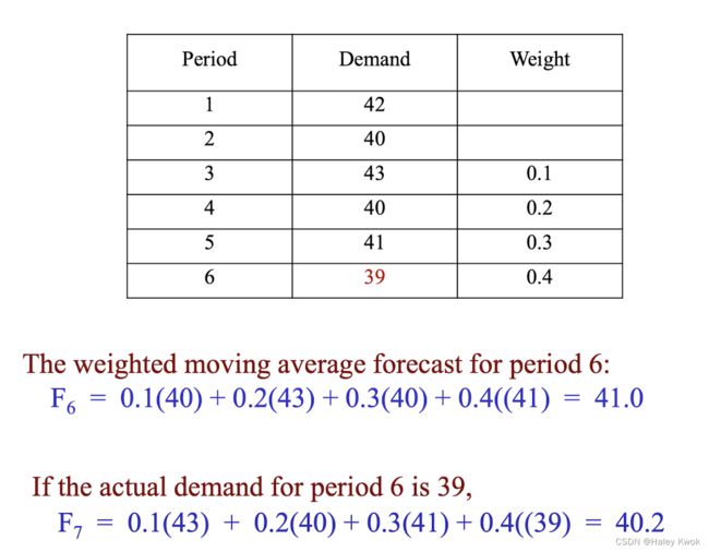
2) Weighted moving average
It is similar to moving average
– Except that it is more reflective of the recent occurrences, (usually it assigns more weight to the most recent values in a time series.)
– The weights must sum to 1.00.
3) Exponential Smoothing
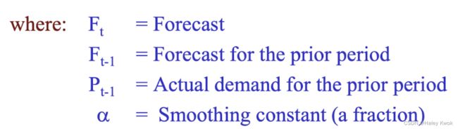
A weighted average method based on the previous forecast plus a fraction/percentage (alpha) of the difference between that forecast and the actual demand of the period.
ie: The forecast for any period = The forecast for the prior period + A fraction of the error in the forecast for the prior period.
Equation used for forecasting:
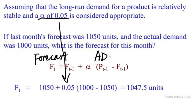
F t = F t − 1 + α ( P t − 1 − F t − 1 ) F_t = F_{t-1} + \alpha (P_{t-1} - F_{t-1}) Ft=Ft−1+α(Pt−1−Ft−1)
An equivalent formula:
F t = α P t − 1 + ( 1 − α ) F t − 1 F_t = \alpha P_{t-1} + (1-\alpha) F_{t-1} Ft=αPt−1+(1−α)Ft−1

Interpretation: the demand during 1 and 2 increases, while the forecast for next period remain the same, showing that the chosen alpha value is not sensitive enough to the changes.
Choice of alpha value
alpha can be between >0 to <1.
Higher the alpha value, greater the weight given to the recent demands.
Commonly used values range from 0.1 to 0.5

Mean Absolute Deviation (MAD)
Error = Actual - Forecast
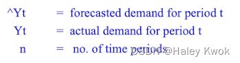
M A D = ( ∑ ∣ Y t − Y t ∣ ) / n MAD = ({\sum} |Y_t - ^ Yt| ) /n MAD=(∑∣Yt−Yt∣)/n
Bias
A measure of the tendency to consistently over or under forecast (error). It is an indication of the directional tendency of forecast errors.
M A D = ( ∑ Y t − Y t ) / n MAD = ({\sum} Y_t - ^ Yt) /n MAD=(∑Yt−Yt)/n
The value of alpha = 0.3 is chosen because of the smaller MAD and Bias resulted.

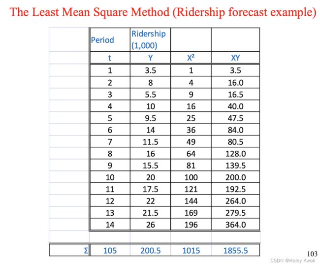
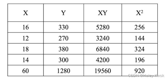
**Least Mean Squares Method
It is a method for trend analysis which involves developing an equation that will suitably describe a linear trend.

Y t = a + b t Y_t = a + bt Yt=a+bt
To determine a and b:
N = No. of data
∑ Y = N a + b ∑ t {\sum}Y = Na + b {\sum}t ∑Y=Na+b∑t
∑ t Y = a ∑ t + b ∑ t 2 {\sum}tY = a {\sum}t + b {\sum}t^2 ∑tY=a∑t+b∑t2
Examples: 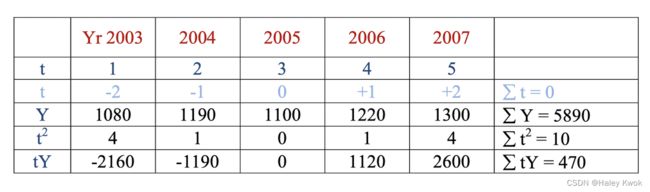
∑ Y = N a + b ∑ t {\sum}Y = Na + b {\sum}t ∑Y=Na+b∑t
5890 = 5a + b (0)
a = 1178
∑ t Y = a ∑ t + b ∑ t 2 {\sum}tY = a {\sum}t + b {\sum}t^2 ∑tY=a∑t+b∑t2
470 = 0 + 10b
b = 47a = 1178 x 1000 = 1178000
b = 47 x 1000 = 47000
Yt = 1178000 + 47000tForecast for the year 2008 (t = 3):
Yt = 1178000 + 47000t
= 1178000 + 47000 x 3
1319000//
Determination of the Seasonal Component
Multiplicative Seasonal Method
It adjusts a given forecast by multiplying the forecast by a seasonality factor.
Seasonal Factor: The index of the “average” periodic demand that occurs in each period.
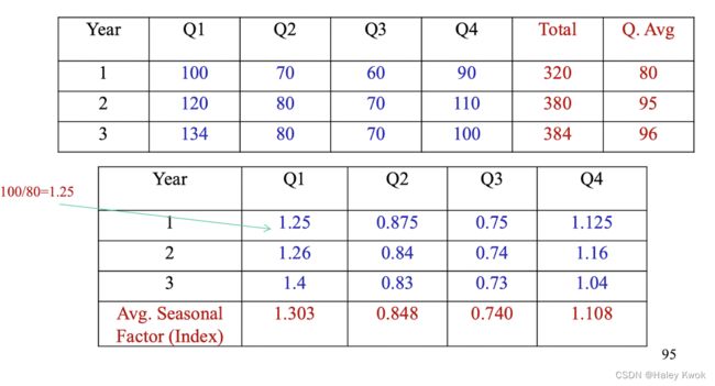
Example: The “Quarterly Average Method”
Quarterly Seasonality Factor = Quarterly demand / Quarterly average

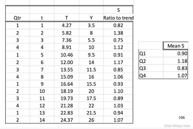
Example: The “Ratio to Trend Method”
Adjusted the forecast by seasonal factors
We can compute, say, for each available quarter of data, a measure of the “seasonality” in that quarter by
S = Y i / Y i S = Yi/ ^Yi S=Yi/Yi


Determination of mean seasonality index
Seasonality adjusted forecast for periods 15 to 18 are

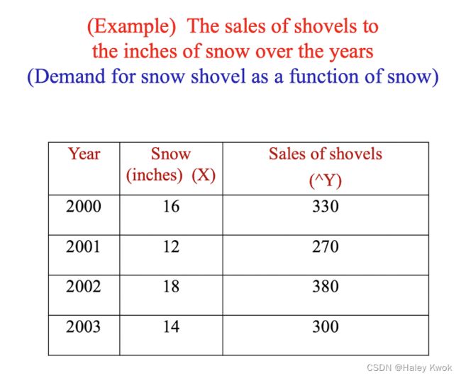
2) Causal Model
Here, the variables which are related to the entity to be predicted are delineated, and their predictive relationship to it is modelled and used for forecasting.
Here, the factors (independent variable) that cause the demand (dependent variable) are being identified and used to forecast the demand.
Simple Linear Regression
The least mean square method used in the preceding section
can also be used to estimate a predicting equation for a
demand in future:
Y = a + b ^Y = a + b Y=a+b


Multiple Linear Regression
The linear regression methodology can be extended to
situations where more than one variable is used to explain
the behaviour of the dependent variable Y.
3) Econometric models
The dependent and independent variables used in forecasting models are interdependent. (e.g., the demand may be a function of personal income and personal income a function of demand, etc…)
Forecast Accuracy and Control
Accuracy: the extent to which the forecast deviates from the actual value
Error = Actual - Forecast
- Mean Absolute Deviation (MAD)
M A D = ( ∑ ∣ Y t − Y t ∣ ) / n MAD = ({\sum} |Y_t - ^ Yt| ) /n MAD=(∑∣Yt−Yt∣)/n
- Bias
M A D = ( ∑ Y t − Y t ) / n MAD = ({\sum} Y_t - ^ Yt) /n MAD=(∑Yt−Yt)/n
- Mean square error (MSE)
[ ∑ ( Y t − Y t ) 2 ] / ( n − 1 ) [{\sum} (Yt - ^Yt)^2] / (n-1) [∑(Yt−Yt)2]/(n−1)
- Mean absolute percent error (MAPE)
[ ∑ ( Y t − Y t ) 2 ] / ( Y t ) ∗ 100 [{\sum} (Yt - ^Yt)^2] / (Yt) * 100 [∑(Yt−Yt)2]/(Yt)∗100
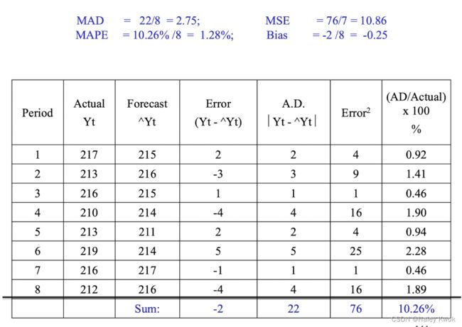
MAD is easiest to compute, but weights errors linearly.
MSE squares errors, thereby giving more weight to larger
errors which typically cause more problems.
MAPE are used when there is a need to put errors in
perspective. (eg, an error of 10 in a forecast of 15 is huge. Conversely, an error of 10 in a forecast of 10,000 is insignificant. Hence to put errors in perspective, MAPE would be used.)
Correlation analysis
It examines the degree of relationship between variables.
Coefficient of determination ( R)
A measure of the proportion of the total variation that is explained by the regression line.
R = 1 − ( [ ∑ ( Y i − Y i ) 2 ] / [ ∑ ( Y i − m e a n o f Y ) 2 ] = r 2 R = 1 - ([{\sum} (Yi - ^Yi)^2] / [{\sum} (Yi - mean of Y)^2] = r^2 R=1−([∑(Yi−Yi)2]/[∑(Yi−meanofY)2]=r2
Coefficient of correlation ( r)
The degree of relationship between variables. r = -1< r < 1
r = 1 − [ ∑ ( Y i − Y i ) 2 ] / [ ∑ ( Y i − m e a n o f Y ) 2 ] r = \sqrt {1 - [{\sum} (Yi - ^Yi)^2] / [{\sum} (Yi - mean of Y)^2]} r=1−[∑(Yi−Yi)2]/[∑(Yi−meanofY)2]

MAD: Forecast Control using “Tracking Signal” method
Forecasting is an ongoing process
Control must be exercised in order to ensure that the technique is working
If it is not, the technique must be adjusted or a new technique be used.
Tracking Signal: The ratio of the cumulative forecast error to the
corresponding value of MAD
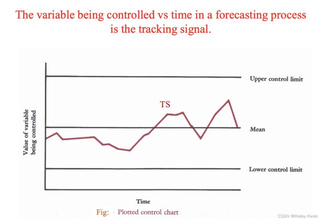
T S ( t ) = R S F E ( t ) / M A D ( t ) TS(t) = RSFE(t)/ MAD(t) TS(t)=RSFE(t)/MAD(t)
T S ( t ) = ∑ ( Y i − Y i ) / M A D ( t ) TS(t) = {\sum}(Yi - ^Yi) / MAD(t) TS(t)=∑(Yi−Yi)/MAD(t)

For RSFE(t),
If the error in a given period is positive, the RSFE will increase,
If the error is negative, the RSFE will decrease.
If the forecasting technique is unbiased, RSFE will be near zero. An unbiased forecast means that the forecast is neither projected too high or too low.

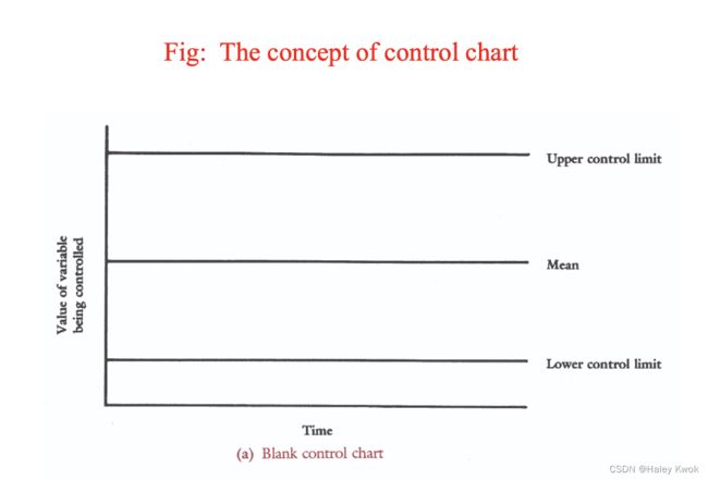
In order to use the tracking signal properly, it is necessary to set up a control chart.
The control chart below represents a 95% confidence control chart.
From the graph, the green line shows the RSFE(t)/ MAD(t); while the red line show the upper and lower control, i.e., t -2 -1 0 1 2
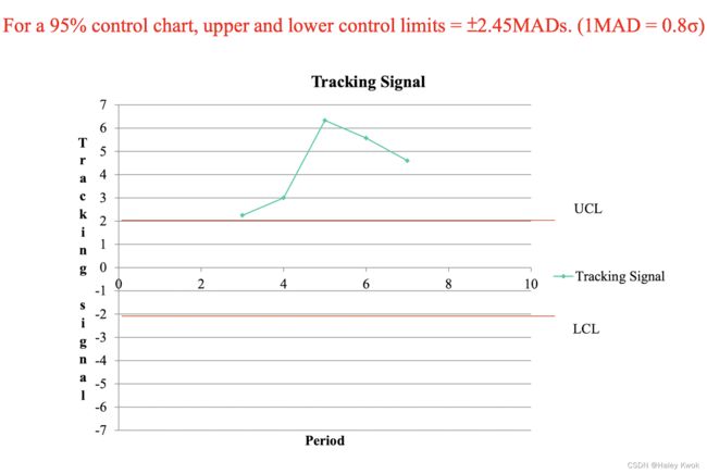
All fall above the UCL, which is very dangerous!
Chapter 4: Aggregate Planning 总体规划
Forecasts are made to project customer demands over a planning horizon.
Then, the company’s resources (capacity, material and
others) must be planned so that,
- the right items/services are produced at the right
quantity, right quality and at the right time - to meet demands of customers over the periods in the planning horizon.
Seasonal variations in demand are quite common in many industries and public services. (air-conditioning, fuel,
travel, police and fire protection.)
Make decision on output rate, employment levels and changes, inventory levels and changes, back orders, and subcontracting, etc -> to deal with the demand variations.
Aggregate Planning V.S. Capacity Planning
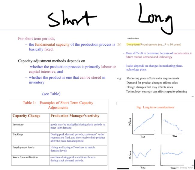
Capacity Planning is about long range capacity that can be changed (add, subtract, remains the same) as planned.
Aggregate Planning is about the utilization of current capacity to satisfy/match aggregate demands over the intermediate time horizon.
Current capacity is not subject for significant change
1. Levels of Capacity Planning
- “Long-range” Planning (say, several to many years)
It is related to product and service selection, facility size and location, equipment decisions, work system design, etc.
- “Intermediate-range” Planning (say, one month to a year or
more)
It is related to level of output, level of employment, and inventories, etc
- "Short-range” Planning (say, a day to possibly a month or so)
It relates to machine loading, scheduling of jobs, workers and equipment.
2. Relationship of Scheduling Activities
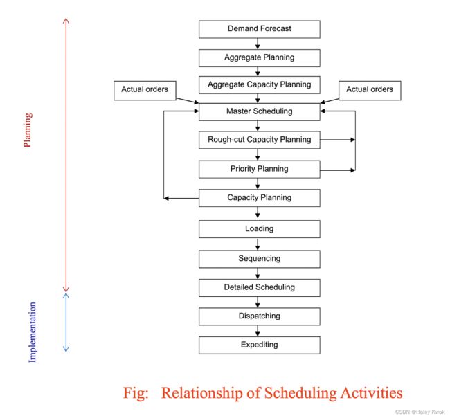
From longest time horizion to shortest time horizion:
- Aggregate Planning: A plan that that basing on the guideline of the business plan, transforms forecasts into programs of activity to produce the aggregate outputs to satisfy the forecasted demand.
3. The Concept of Aggregation
It involves combining the relevant resources/outputs into overall aggregates (such as the total work force, output, and inventory).
It represents the plan for production across a family or product line that uses the same resources.
Aggregate output: Volume of products produced • Barrels of oil in the oil industry • TVs, cars produced • Hours of service provided • Number of patients seen • Number of beds in a hospital
Aggregate resources: total number of hours of workers (man-hours) • total number of hours of machine time (machine-hours) • total weight of raw materials • Total number of consultant-hours
Master Scheduling (Disaggregation)
A plan showing the time phased quantities and date for each item to be produced.
An aggregate plan must be disaggregated into planned production levels for individual products in each period (eg., month).

Master Production Schedule (MPS)
- disaggregates the aggregate plan into scheduled production levels of individual end products.
- provides the end-item production quantities and dates of the production.
Material Requirement Planning (MRP)
A system for planning the materials that are required to produce the quantities and items specified in the master production schedule.
Loading
Deciding which jobs are to be assigned to which work centre in a planning period.
Sequencing
To decide the order in which the jobs are to be performed on an equipment or by a work person.
Scheduling
The drawing up of detailed schedules itemizing specific jobs, times, equipment, materials, and workers.
Dispatching
Starting off of the production orders
4. Aggregate Production Planning
Aggregate planning is about the utilization of current capacity (plant, equipment, and manpower) over the intermediate time horizon to effectively satisfy aggregate demands in the period.
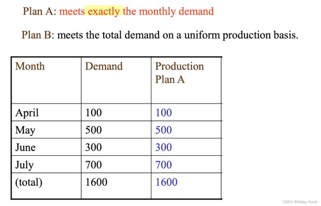
4.1 A pure strategy
means that output is changed by varying only one of the variables at a time.
Demands in Feb and Mar are respectively 100 and 300 units
Assuming no. of employees in Jan was 20. (Output/man=10 units) (Layoff cost= $400/employee; Hiring cost= $300/employee)

Examples
- Vary the size of the work force. (hire and layoff)
- Carry finished goods inventory.
- Utilize overtime.
- Add extra shifts.
- Vary the load by altering the product mix.
- Subcontract work to other firms (the make or buy decision).
- Vary the level of customer service.
- Add contra-cyclical (complementary) products to stabilize demand.
- Vary marketing (price, advertising) to counter-influence the demand
pattern.
Modify capacity
- Work study to improve work methods
- Training
- Better utilization of resources,
eg, better scheduling, preventive maintenance, etc
Modify output
Eg:
• Product/service standardization
• Have the customers do part of the works
• Make to stock rather than make to order
Steps in Aggregate Planning
- Determine organizational policy regarding controllable variables.
- Establish the forecasting time period and the horizon of the production plan.
- Develop the demand forecasting system.
- Select an appropriate unit of aggregate capacity.
- Determine the relevant cost structures.
- Use an appropriate production planning method.
- Develop alternative plans and determine the cost of each. 8. Select the plan that best satisfy the objectives (eg, least cost)
4.2 Planning Strategy
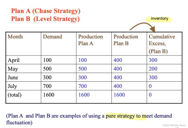
4.3 Chase strategies
One that matches demand during the planning horizon by varying the output rate by, eg:
– The workforce level (Hiring and layoffs)
– Over-time,
– Under-time,
– vacation/plant closure arrangements,
– subcontracting, etc
4.4 Level Strategies
One that maintains during the planning horizon,
– a constant workforce level,
– a constant output rate.
4.5 A mixed strategy
means that output is changed by varying two or more of the variables at a time
Exactly matches demand for certain periods but runs shortages for other periods;
Runs a small inventory the first two quarters and then a small shortage the last two quarters,
Example 1
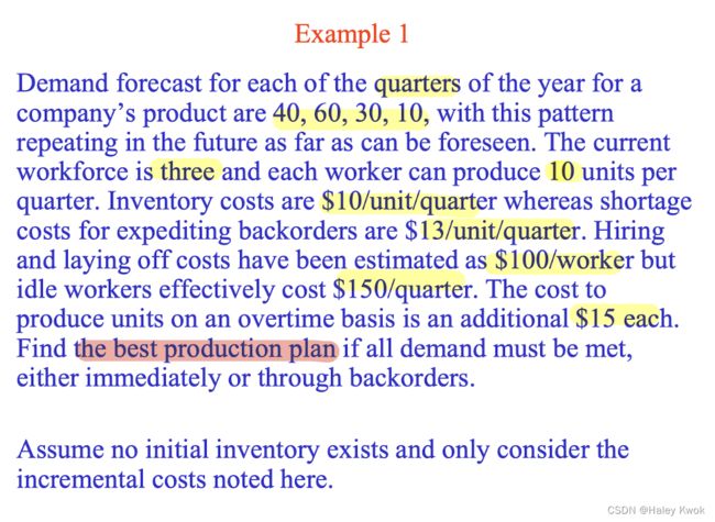
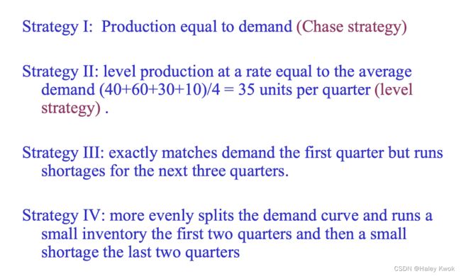
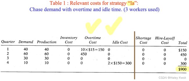
Strategy 1: Chase Strategy

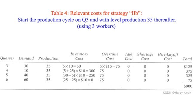
Strategy 2: Level Strategy

Strategy 3:
Strategies III: produce 40,40,40,20 (use 4 workers)
Strategy 4:
Strategy IV: produce 50,50,20,20 (use 4 workers)

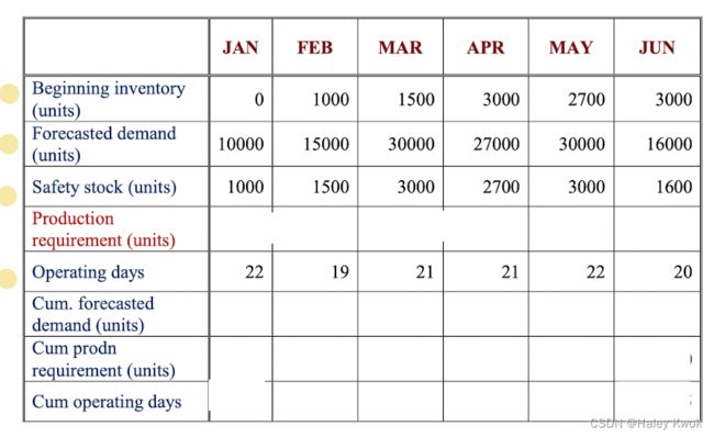
Example 2
You are supplied with:
– a monthly demand forecast,
– an organizational policy of requiring 10% of a month’s
forecast as safety stock, and
– the number of operating days available each month. (* workers work 8 hrs a day)
There is no inventory available at the beginning of the first month, January.
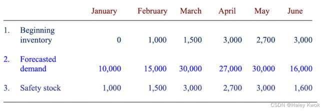


Steps: input the given information:

Three potential plans for the production are:
- Produce to exact production requirements
(chase strategy)by varying the size of the work force on regular hours. Assume there are 250 men available in January.
22 days * 8 hours

- Maintain a constant work force of 518 men
(level strategy). Assumeno subcontractingis available and inventory will fluctuate withstockoutsfilled from the following month’s production.

- Produce with a fixed work force of 500 men on regular time
(level strategy)andsubcontractall excess demand over the period production. Inventory will increase when production exceeds demand.No stockoutsare permitted.

Methods of Aggregate Planning
ii) Production Plan Spread Sheet (PPSS)
• The PPSS basically lays out the production plan for the next several months.
• It considers production on regular time, overtime, and subcontracting for each month.
• For a given work force size, the PPSS can determine the optimum production levels for each month.
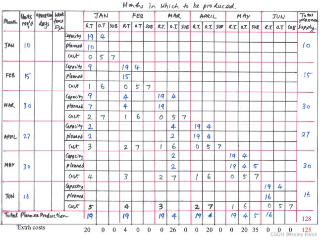
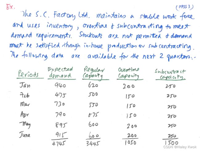
Example 1 (PPSS):
An organization uses overtime, inventory, and subcontracting to absorb fluctuations in demand.
A production plan for 6 months is devised and updated each month.
The expected demand for the next 6 periods is as follows:

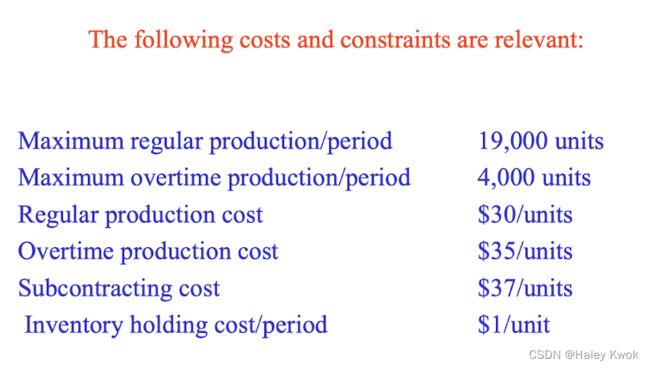
Using a PPSS:
Obtain the optimum production plan for the next 6 months (assume beginning inventory is zero, desired ending inventory is zero, and no stockout can be tolerated).
Example 2

Aggregate Planning
Linear Regression
Detailed demand
MRP, MPS
Chapter 5: Master Production Planning – Master Production Schedule (MPS)
Aggregate Planning represents production across a family or product line that uses the same resources. To be useful for actual production planning
- This must be broken down (disaggregated) on a product-by-product basis into a Master Production Schedule.
It is this point (master scheduling) that actual orders are incorporated into the scheduling system.
- For production to order
The master schedule may be developed strictly from the order backlog or from a combination of the order backlog and a forecast. - For production to stock
The master schedule is developed from a demand forecast.
The schedule is then checked against lead time (time to produce or ship the items) and operations capacity for feasibility. (rough cut capacity planning)
Aggregate Planning V.S. Master Scheduling
The MPS might be divided by time fences at 2, 2, 4 and 8 weeks to specify the degree of change permitted:
- Frozen: the first 2 weeks (no change allowed)
- Firm: the next 2 weeks (only minor changes allowed)
- Flexible: the next 4 weeks (somewhat greater changes allowed)
- Open: After 8 weeks, schedule is open, any changes are allowed
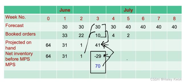
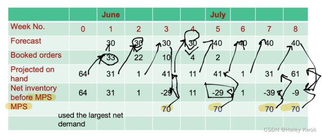
Production Lot Size:
When future demand for an end item can be anticipated, an economic production lot size may indicate a minimum production quantity.
– If demand exceeds the economic lot size,
• the larger quantity is produced.
– If demand is less than the economic lot size,
• the excess quantity can be placed in inventory for future requirement.
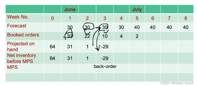
We always consider the largest net demand. In week 3, we only got 1 project on hand, while having 30 forecast, that’s not enough. Then we make MPS by considering all situations, we should have 30+10+1 = 41, then consider -29 back-order, we need 70 in total.
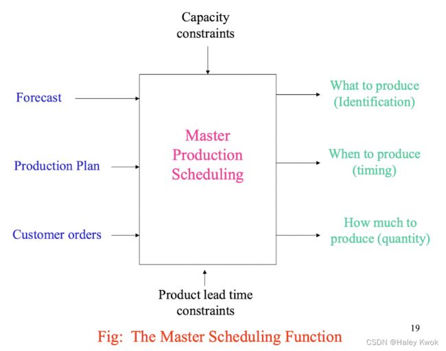
Capacity and Priority Planning
Priority planning
– determines the order (timing) in which goods are produced.
– (When a product is to be produced?)
Capacity planning
– determines what type of labour and equipment capacity
is required and when it is required.
– (Do we have the capacity?)
Capacity Requirement Planning (CRP)
– The process of determining workloads on each of the work centers due to the Master Production Schedule of final products.
– The capacity and delivery lead time must be checked for feasibility before the master schedule can be finalized
A master schedule must be realistic
– Capacity limits must be carefully observed.
– If demands exceed resources,
• reduce the master schedule or
• increase resources (capacity).
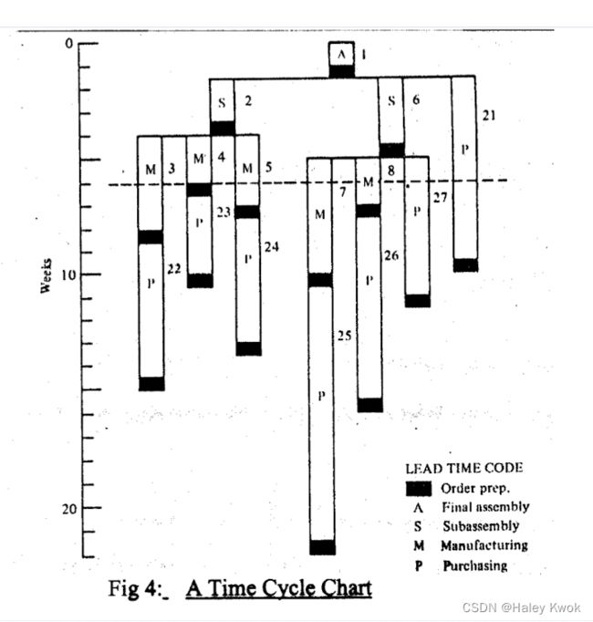
Time Cycle Chart
• It shows how much time it would take to produce a product starting from scratch with no inventories available.
• It indicates lead time requirements as well as the minimum planning horizon for the master schedule.
If customer delivery is to be made in less than the maximum time on the time cycle chart,
– what can we do?


• In the make to stock environment:
– The MPS is based on the finished products.
• In the assembly to order environment:
– The MPS is at the modular or subassembly level.
– The final assembly will be based on product bills.
• In the make to order environment:
– The MPS is based on the component/raw material level.
– The final assembly is based on the product bill
Master Schedule Revision
A master schedule should be an up-to-date rolling schedule that is revised by adding periods and updating as necessary.
– As new information or new orders become available, the schedule will change.
– At the end of a period, any incomplete work must be rescheduled.
When properly maintained, a master schedule can reduce inventory, improve customer service, and increase productivity.
Chapter 6: Inventory Management and Control
As inventory may represent a significant portion of total assets of a company,
– A reduction of inventory can result in a significant increase in its ROI (Return on Investment).
– Good inventory management is important for the successful operation of businesses.
Principle Kinds of Stocks
- Finished goods
- Act as a cushion (buffer) between supply and demand.
- Enable the firm to meet orders promptly.
- Work in progress (WIP) (Partially completed goods)
- To decouple production operations. (Maintain independence of production operations.
- Raw materials and purchased parts. (including replacement parts, tools and supplies)
- Protect against disruptions of supply/delivery
- Take advantage of economic purchase order size.
- Quantity discounts
Purchase supplies at advantageous prices
- Hedge against price increase
Facilitate steady and efficient plant operation
- Protect against demand fluctuation
Buffer stock (safety stock):
– to act as a buffer against fluctuation in demand.
Strategic stock:
– the additional stock needed to allow for delay in delivery or for any above average demand that may arise during the lead time.
Lead time:
– the time between deciding to place an order and receipt of replenishment.
Stock costs
Too low a stock level: loss of business or high production cost.
Too high a stock level: tie up capital with no direct return.
1. A typical inventory control system
- Development of demand forecast.
- Selection of inventory models.
- Measurement of inventory costs.
- Methods used to record and account for items.
- Methods for receipt, handling, storage and issue of items.
- Information procedures used to report exceptions
2. Stock Control Systems
1) The fixed reorder quantity system
fixed order quantity system (order at different time period, while Q is fixed)
a) The maximum and minimum ordering system
buy exactly the same amount, make the fixed quantity; which means when you have the Q order, you use your stock, and it goes back to 0 again, and placed new order

a) The maximum and minimum ordering system (with safety stock)
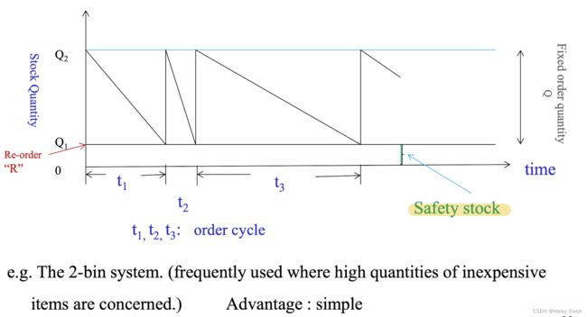
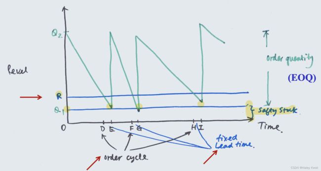
b) Perpetual Inventory System
+R+lead time
variable demand, fixed reordering point R, fixed ordering quantity Q (EOQ), fixed lead time, variable order cycles.
whenever go to R, triggers you to reorder, but why not there is inventory directly? It is because there is lead time {D-E, F-G, H-I}
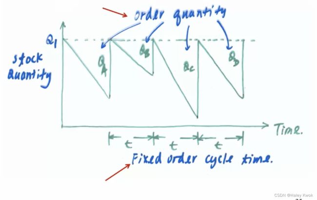
2) The order cycle system (the fixed reorder interval system)
fixed order cycle system (order at fixed time period, while Q vary)
Orders are made at fixed intervals and of a size calculated to bring stocks up to a fixed level at the time of delivery.
Advantage:
– Facilitate administrative works.
– Also, suppliers know when the orders are to be received and thus can prepare for them accordingly.
Review at fixed time interval, Q varies in each time period
Optional Replenishment Inventory System (with reorder point)

3. Material Requirement Planning (MRP)
a) A derived order quantity system for dependent materials and items used to produce an end item.
– It is a quantity based; time based and production based planning system
b) It functions by working backward from the scheduled completion dates of end products
– to determine the dates and quantities of the various component parts and materials that are to be ordered.
c) Extensively used with planned production.
– Usually administered by a computer with appropriate MRP , MRPII and ERP packages.
4. Economic Order/Batch Size (EOQ)
A) For Raw Materials, WIP and Final Inventory
- Setup cost (ordering cost):
a) The cost of ordering and receiving inventory.
b) The cost incurred every time equipment and facilities are prepared for the manufacture of an item
c) Unit direct labour costs: The “learning effect” leads to decrease in unit labour cost for larger production runs.
[Example]
• Administration cost (invoicing, shipping, inspection, material handling, etc)
• Cost of setting up the machine
• Cost of new jigs and tools
• Wastage cost, etc.
- Stock Keeping Costs(holding costs) (Related to physically holding stocks in storage)
[Example]
a) Deterioration costs
b) Obsolescence costs
c) Insurance and storage costs
d) Loss of return on capital
- Shortage Costs
Costs resulted when demand exceeds the supply of inventory on hand
[Example]
a) Loss of not making a sale.
b) Late delivery penalty
c) Loss of Customer goodwill.
d) Cost of lost production’
e) Cost of machine downtime
B) For Purchased Items:
- Quantity discount:
– achieved only at the cost of increased stock levels.
D: discount per piece
K 1 K_1 K1: cost of stock holding per unit of time per piece
T: time
Q: quantity of stock (pieces)
If the saving through large quantities purchase is greater than the additional cost of store keeping, policy “a” is preferred, ie:
If 3Q (D) > [0.5(3Q) - 0.5 (Q)] K 1 K_1 K1T

5. Economic Order/Batch Quantity
Objective: to minimize the total costs related to stock keeping
Critical cost components:
C = C s + C 1 + C 2 + C 1 C = C_s + C_1 + C_2 + C_1 C=Cs+C1+C2+C1
C = total critical costs / yr
C s C_s Cs = order set up costs / yr
C 1 C_1 C1 = stock carrying costs / yr
C 2 C_2 C2 = shortage (underage) costs / yr
C 1 C_1 C1 = cost of inventory kept / yr
The decision consists of:
For the stock keeping unit (SKU) you want to keep:
- How much to order (or produce)? (EOQ, EBQ, EMBQ)
- When to order (the reorder point R)?
Model I
Assumptions: Demand constant and known. No shortage allowed. Zero purchase lead time. No safety stock.
Let: K S K_S KS = set up cost per batch
K 1 K_1 K1 = holding cost per item per unit of time
K 2 K_2 K2 = shortage (penalty) cost per item per time
To supply D items at a constant rate in time T:
q = batch size (units)
t = time between runs = T * (q/ D)
Assuming average stock level = q/2
Inventory holding cost = q/2 K 1 K_1 K1 t per batch
Total inventory cost per batch = q/2 K 1 K_1 K1t + K s K_s Ks
Total cost per time T = (q/2 K 1 K_1 K1T + K s K_s Ks D/q) = ( K 1 T q ) / 2 + ( K s D ) / q ({K_1}Tq)/2 + ({K_s}D)/q (K1Tq)/2+(KsD)/q, where
( K 1 T q ) / 2 ({K_1}Tq)/2 (K1Tq)/2 = holding cost
( K s D ) / q ({K_s}D)/q (KsD)/q = setup cost
Total cost must have a minimum value since holding cost is proportional to q, while setup cost is proportional to 1/q

Find the optimum batch size q o p t q_{opt} qopt
After differentiation,
For the minimum cost:
( K 1 T ) / 2 = ( K s D ) / q 2 q o p t ( E O Q ) = ( 2 K s D ) / K 1 T C o s t ( m i n ) = 2 K s D K 1 T (K_1 T)/2 = (K_s D)/ q^2 \\ q_{opt}(EOQ) = \sqrt{(2K_s D)/K_1 T} \\ Cost(min) = \sqrt{2K_s D K_1 T} (K1T)/2=(KsD)/q2qopt(EOQ)=(2KsD)/K1TCost(min)=2KsDK1T
The Economic Reorder Point ( R)
R = L T ∗ U R R = L_T * U_R R=LT∗UR, where
L T L_T LT = lead time (number of days)
U R U_R UR = utilisation per day
R = L T ∗ U R + Q S R = L_T * U_R + {Q_S} R=LT∗UR+QS, where there is safety stock to be maintained
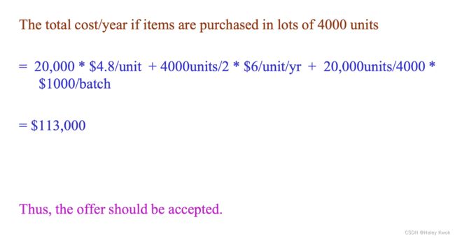
Quantity Discounts
C = C s + C 1 + C 1 C = C_s + C_1 + C_1 C=Cs+C1+C1
Let C 1 = K p D C_1 = K_p D C1=KpD , where ( K p K_p Kp = price/unit)
C = K s ∗ D / q + K 1 ∗ q / 2 ∗ T + K p D C = K_s * D/q + K_1 * q/2 * T + K_p D C=Ks∗D/q+K1∗q/2∗T+KpD
[Example]

A1 : use EOQ
A2 : stock 201 for a 5% discount
A3 : stock 401 for a 10% discount
C = K s ∗ D / q + K 1 ∗ q / 2 ∗ T + K p ∗ D C = K_s * D/q + K_1 * q/2 * T + K_p * D C=Ks∗D/q+K1∗q/2∗T+Kp∗D
(EOQ = 160 units)
Cost for A1 = 40800
A2 = 38820.90
A3 = 37161.35 -> selected
[Example]


Model II

Holding cost = K 1 ∗ S 2 / 2 Q {K_1 * S^2} / 2Q K1∗S2/2Q
Shortage cost per unit of time = K 2 ( Q − S ) 2 / 2 Q {K_2 (Q-S)^2} / 2Q K2(Q−S)2/2Q
Setup cost per unit of time = K s / ( Q / r ) {K_s} / (Q/r) Ks/(Q/r), where r = rate of usage
W i t h o u t s h o r t a g e : Q o p t ( E O Q ) = ( 2 D ∗ K s ) / K 1 ∗ T W i t h s h o r t a g e : Q o p t ( E O Q ) = ( 2 D ∗ K s ) / K 1 ∗ T ∗ ( K 1 + K 2 ) / K 2 C o s t ( m i n ) p e r y e a r = 2 ∗ K S ∗ D ∗ K 1 ∗ T ∗ K 2 / ( K 1 + K 2 ) N O T S U R E A B O U T T H I S : S = ( 2 D ∗ K s ) / K 1 ∗ T ∗ K K 2 / ( K 1 + K 2 ) Without shortage: Q_{opt} (EOQ) = \sqrt{(2D * K_s)/ K_1 * T} \\ With shortage: Q_{opt} (EOQ) = \sqrt{(2D * K_s)/ K_1 * T} * \sqrt{(K_1 + K_2) / K_2} \\ Cost (min) per year = \sqrt{2 * K_S * D * K_1 * T} * \sqrt{K_2 / (K_1 + K_2)} \\ NOT SURE ABOUT THIS: S = \sqrt{(2D * K_s)/ K_1 * T} * \sqrt{KK_2 / (K_1 + K_2)} Withoutshortage:Qopt(EOQ)=(2D∗Ks)/K1∗TWithshortage:Qopt(EOQ)=(2D∗Ks)/K1∗T∗(K1+K2)/K2Cost(min)peryear=2∗KS∗D∗K1∗T∗K2/(K1+K2)NOTSUREABOUTTHIS:S=(2D∗Ks)/K1∗T∗KK2/(K1+K2)
[Example]

6. Pareto Analysis (ABC classification) of stock items
Pareto Analysis
It is generally observed that for many events, roughly 80% of the
effects come from 20% of the cause
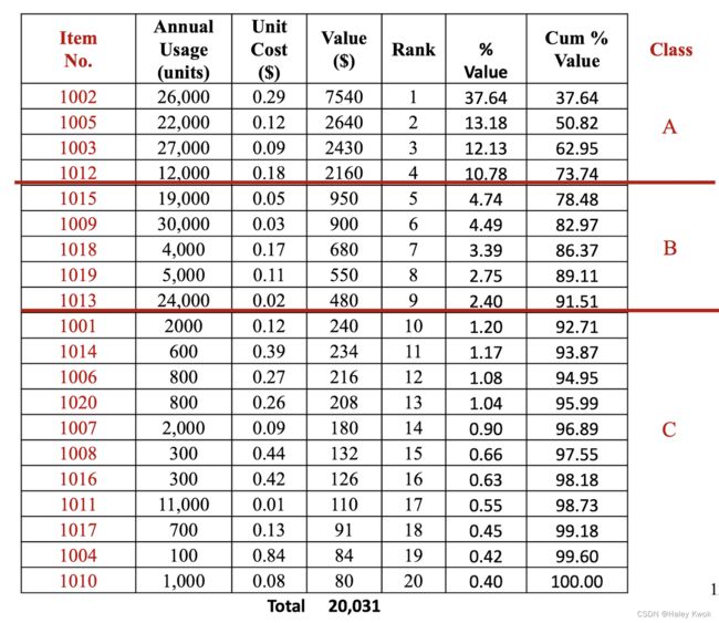
ABC Classification
- Class A : Very Important Items. (whose dollar volume typically accounts for 75- 80% of the value of the total inventory, while representing only 15- 20% of the inventory items. )
- Class B : Moderately Important Items. (where dollar volume accounts for 10- 15% of the value of the inventory, while representing 20- 25% of the inventory items. )
- Class C : Least Important Items. (whose volume accounts for 5 -10% of the inventory value but 50- 60% of the inventory items.)
ABC (Pareto) Analysis
A method used to divide inventories into say three classes according to dollar usage (e.g. unit purchase cost or production cost, holding cost, etc.)
- The inventory value for each item is obtained by multiplying the annual demand by the unit cost.
- The entire inventory is listed in descending order from the largest to the smallest.
- The items are then designated by the ABC classification system
Selective inventory control
Inventory management may involve thousands of items, and even millions of individual transactions each year.
A Materials Manager must identify those items that require
precise control from those that do not.
- Class A : Receives greatest attention. (High Value Items)
e.g. EDQ developed with a review of the variables each time an order is placed. (Perpetual system used) - Class B : Receives medium level of attention. (Medium Value Items) e.g. EDQ developed with a semiannual review of its variables. (Periodic system used)
- Class C : The least attention received. (Low Value Items)
e.g. needs no special calculation. Order quantity might be one-year supply with periodic review once a year. ( eg. 2- bin system used)
Advantages
- Holding cost will be reduced
- Floor space will be available for manufacture rather
than for storage - More cash will be available for use in other ways
- Reduction in administration and clerical effort
Chapter 7: Material Requirements Planning (MRP)
Relationship of Scheduling Activities

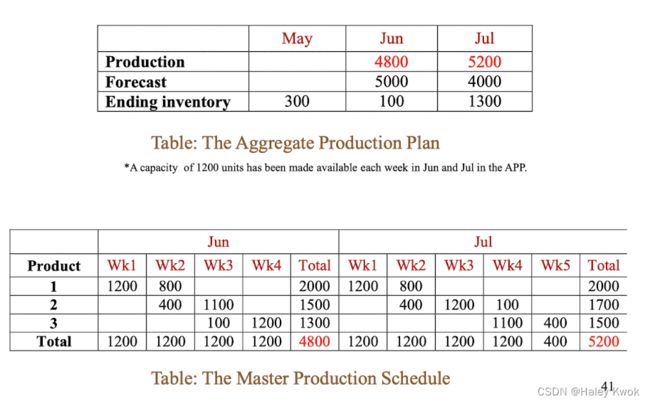
Example: Master Scheduling based on the Aggregate Production Plan previously drawn
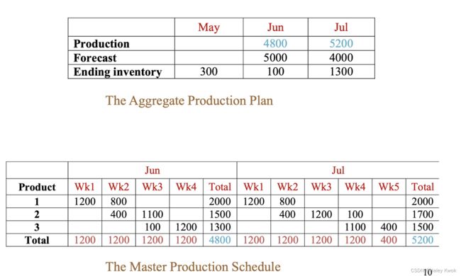
The next level of disaggregation can be MRP:
- MRP is used to time-phase and schedule the subassemblies and parts needed to support end item production.
- It translates the finished product requirements of the master schedule into time-phased requirements for subassemblies, component parts and raw materials.
The major objectives of an MRP system are to:
- Plan manufacturing activities, delivery schedules, and purchasing activities
- Ensure the availability of materials, components, and products for planned production and for customer
delivery. - Maintain the lowest possible level of inventory,
Key features of an MRP system
- time phasing of requirements
- generation of lower-level requirements
- planning orders and releases
- rescheduling capability
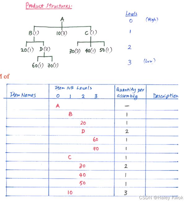
1. Product Structure
- Independent: no relationship exists between the demand for an item and any other item, such as end items or products. (eg. A car, a TV set)
- Dependent: means the demand for an item is the result of the demand for a “higher level” item. (eg., parts and materials that go into production of the car, TV set.)


1.1 Independent demand
The demand for the final product may be continuous and independent

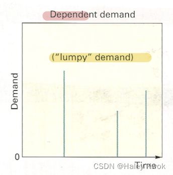
1.2 Dependent demand
The demand for lower-level items composing the final product tends to be discrete, derived, and dependent.
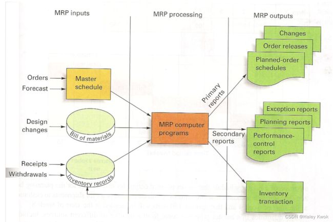
2. MRP Inputs
- Master schedule
MRP takes the master schedule for end items and translates it into individual time-phased component requirements.
Gross requirement =~ MPS
MPS is made in accordance to demand/forecast
-
inventory status records
All inventory items must be uniquely identified.
– Information on
• lead times,
• lot sizes,
• Quantities of items in inventory “on-hand” at the start of a planning horizon that are available for use
• Quantities of items “on-order” that are expected to become available during a planning horizon from open work orders or open purchase orders. -
Product structure
Bills of materials (BOM) records
It contains the BOM for the end items in levels representing the way they are actually manufactured


An Indented BOM of Product A
3. MRP Outputs
Planned Orders: a schedule of orders indicating the amount and timing of future purchase or production of items required in each time period to produce the end items.
Order Releases: release of orders to authorize the execution of planned orders by purchasing and or production shops. (They provide the quantity and time period when ‘work orders’ (WO) are to be released to the shop or ‘purchase orders’ (PO) placed with suppliers.)
The “open order reports”: reports that show which orders are to be expedited or de-expedited.
Summary of MRP
4. The Material Requirement Planning (MRP) Process
MRP takes MPS for end items and determine the gross quantities of the components required from the product structure records.
-
Explosion:
Gross requirement
The exploding process is simply amultiplicationof the number of end items by the quantity of each component required to produce a single end item. -
Netting:
By referring to the inventory status records, the gross quantities are netted bysubtractingthe available inventory items.
Net requirements:
- Positive: an order MUST be schedules to be received in time
- Negative or zero: no order is necessary
Projected on hand: is the expected amount of inventory that will be on hand at the beginning of each time period.
Scheduled receipts (on order): the quantity expected to be received by the beginning of the period.
Gross Requirements for the planning period - Planned On hand at the planning period
- Offsetting:
– Order release dates are determined byoffsetting (setting back in time) the lead timesfor each component
Planned order releases: the releases of the planned amount to order in each time period.
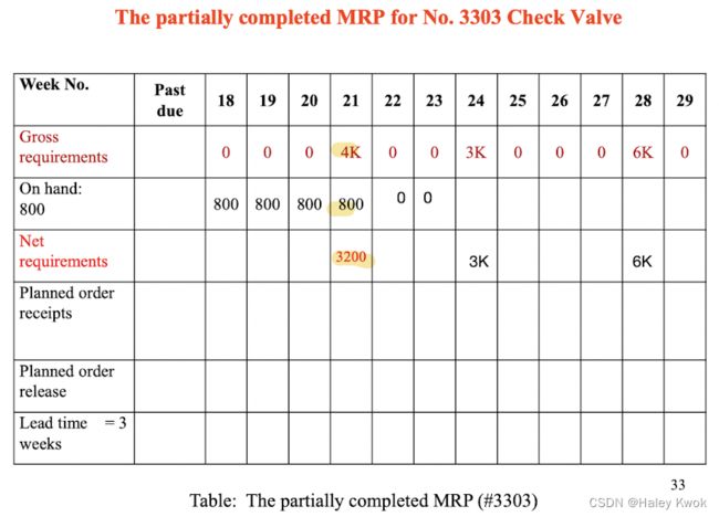
5. MRP Computation
Gross requirement: The total expected demand for an item during each time period without regard to the amount of inventory on hand.
– The quantity that is generated by exploding the bill of materials.
– It does not take into account any inventory status.
Net requirement: The actual amount needed for an item in each time period. (The quantity that must actually be acquired to meet the demand generated by the master schedule. )
Scheduled receipts (on order): the open purchase or work orders scheduled to arrive by the beginning of a period.
Caluculations
For each item at a level:
- Determine the time-phased
gross requirementsby summing planned order releases of its parent items multiplied by the quantity usage rate per parent item, for each period of the planning horizon. - Subtract on-hand and on-order amounts from gross requirements to determine the
net requirements (netting). - Apply the
lot-sizingrule assumed to determine the lot size. Offsetthe order release for lead time, yielding time-phased planned order release.
IMPORTANT COMPONENTS
STEP 1: production structure
STEP 2: projected on hand
STEP 3: | explode from planned order release
STEP 4: <-
STEP 5: lot size: the actual order quantity for an item, where it determines an appropriate (minimum or less cost) lot size for ordering or production.
- Although there is level 1 E is not counted in the level code as level 1, but it does not affect the computation; i.e., there is still E(1) after Q
- projected on hand = planned order receipt - net requirement, where net requirement == gross requirement. Since if there is project on hand, net requirement would be less.
- if projected on hand can fulfil the gross requirement, then we do need to have the planned anymore.
The MRP

Lot sizing
Period order quantity (POQ) Method
The average demand is used to determine EOQ (as approximate order lot size) and rounded to the nearest integer
[Example]
An item that uses “week” as the “time bucket” has an average weekly demand of 138 units, an order cost of $50 per batch, a weekly holding cost of $0.1 per unit. Using the POQ method, determine the ordering quantity and the periods when orders will be placed.
Assuming that the period 5 was the earliest period with a net requirement for this item.
EOQ = 371 units
EOQ/Average demand = 371/138 = 2.69 (rounded up to 3 periods)

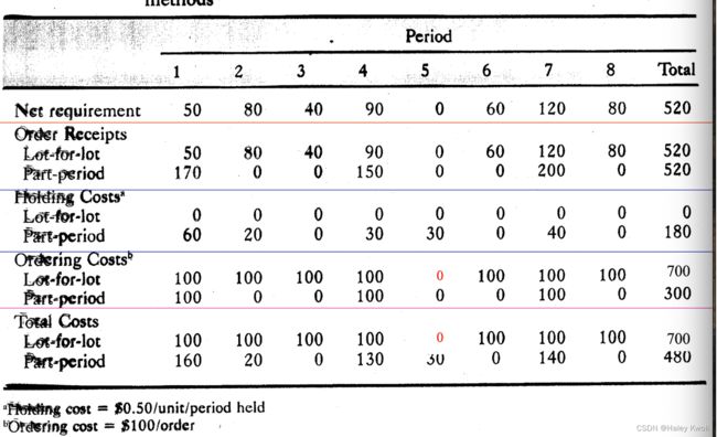
Part-Period Balancing Method


-
The total order set up cost and inventory holding cost for the policy using part period balancing method = 4 batches * $55/batch + 500 units*$0.05/unit/period + 300 units *
*$0.05/unit/period *2 + 800units * $0.05/unit/period +100 units *
$0.05/unit/period + 300 units * *$0.05/unit/period *2 + 200 units *
*$0.05/unit/period = $360 for the 10 periods . -
The total order set up cost and inventory holding cost for the policy
using lot for lot ordering method. = 10 batches * $55/batch = $550 for the 10 period
The Economic Part Period Method (EPP)
Determine the EPP by dividing setup cost by unit holding cost per period.
Eg, if order cost = $55/order & holding cost = $0.05/unit/period, EPP = $50/$0.05 = 1000 units
ERP
The system contains more than MRPII contains and can addresses many functions related to manufacturing and other concerns.
– An ERP also provides tools for planning and monitoring various business processes.
Exercise


Chapter 8: Operations Loading and Scheduling
1. Loading
– The assignment of works to a facility without specifying when each of the work is to be done and in what sequence.
Bar Chart
– A graphical method to show the total estimated work load that the open orders require to be processed on work - centres.
The Gantt (Load) Chart
− A graphical method to visually display the actual and intended use of resources in a time framework.
−depicts the loading and idle times for a group of machines or a list of departments.
Index Method (For Loading Jobs to Machines)
Index: Obtained by dividing the shortest possible processing time of the job into all its respective processing times in the work centres.

2. Scheduling
– the assignment of works to a facility with the time specification and the sequence in which each of the work is to be done.
Master Scheduling
– The planning of the level of production (output) for the total facility.
– The time horizon is usually 3 months to 1 year
Detailed Scheduling
– The planning of the schedule of production at a much lower organizational level.
– It deals with day-to-day operations. It operates within and is confined by the master schedule.
Approaches
-
Forward Scheduling
It starts with the first operation as soon as factors of production are available and works forward by scheduling each succeeding operation until the completion of the last operation is reached.

-
Backward Scheduling
It begins with the desired delivery date and the last operation and works backward by scheduling each preceding operation until the first operation is reached.

Finite Capacity:
– Assign jobs to work centres so as to never exceed their capacities.
Infinite Capacity:
– Assigns jobs to work centres without regard to capacity limitations.
A Gantt (Scheduling) Chart
A time-phased bar chart for displaying the job schedule and
for tracking progress on all components of a job.

3. Sequencing
– the process of setting priorities for works to be carried out on a facility
Sequencing jobs on 2 machines

Johnson’s Algorithm (Sequence jobs for 2 machines)
A method to schedule for minimum total throughput time.
eg: (Jobs pass through m/c 1 and 2 successively for processing. The numbers are times (hr) required to be worked)
- Identify the job(s) with the smallest individual machine
processing time(s). - If the smallest time appears on m/c I, it is done first.
- If it appears on m/c II it is done last.
- The jobs thus scheduled are eliminated &
- Repeated the above till all jobs are scheduled.
– This technique is particularly useful where 2 consecutive m/c are very costly.
Shortest processing time
M1: A
M2: E

[Example]
A company receives parts from suppliers to be used in their production system. The quality control department must perform two operations when shipments are received:
- determine the sequence of processing the shipments through the two operations using the “Johnson’s algorithm”
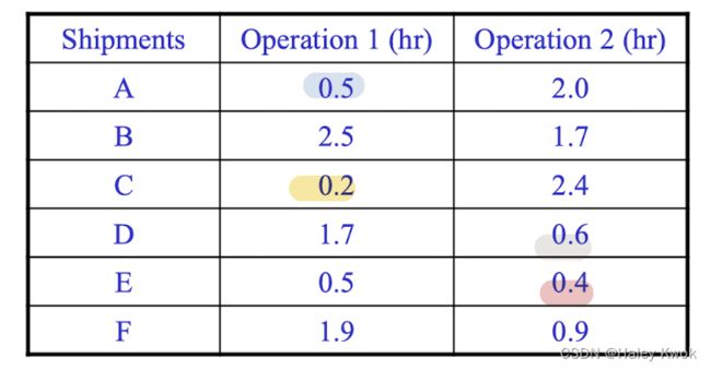
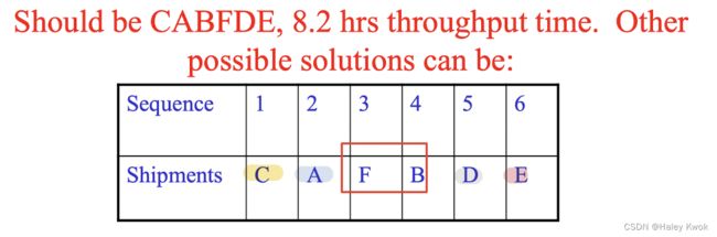
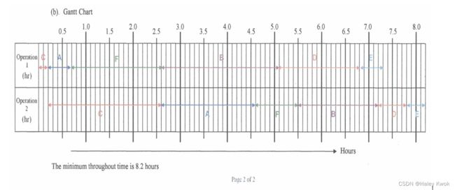
- With the aid of a Gantt chart, find the minimum throughput time (hrs) for completing checking all the shipments
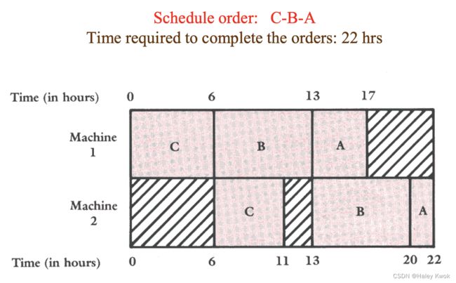
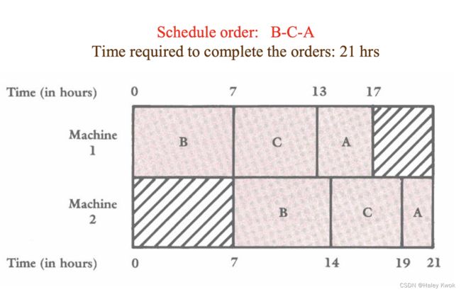
Sequence jobs for 3 machines
Generate a 2 fictitious machine problem, then apply Johnson’s Algorithm.
- The shortest processing time on machine 1 is longer than the longest processing time on machine 2, OR
- The shortest processing time on machine 3 is longer than the longest processing time on machine 2
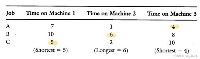
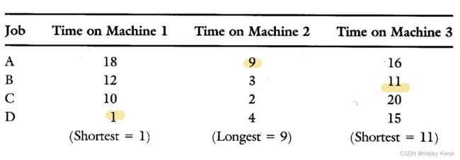
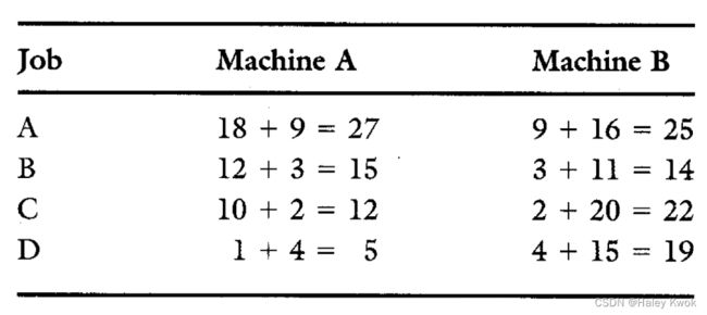
The order is: DCAB. However, this may not be the only best answer. DCBA is also equally good.
Cambell, Dudek and Smith Algorithm (C-D-S Algorithm, for sequencing N jobs to M machines)
It requires the generation of a number of fictitious two-machine schedules, which are then sequenced using the Johnson two-m/c algorithm method.
The sequence which generates the least throughput time is the one likely to be a near minimal sequence.
For scheduling and sequencing of N jobs on M machines:
• Calculate the ‘processing time’ for a series of pairs of fictitious machines M1 and M2.
• For the Kth pair:
– Processing time on M1 = processing time on the first K
machines
– Processing time on M2 = processing time on the last K
machines
(The number of such pairs is M-1)


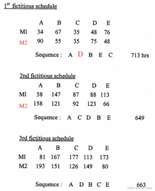
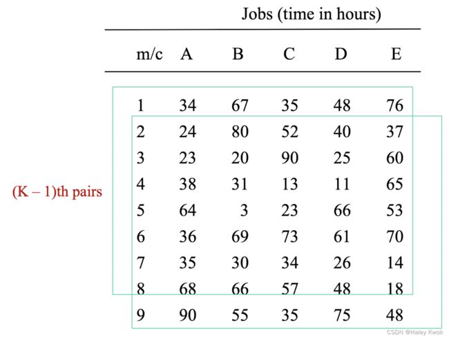

You can see that just add up the whole line.
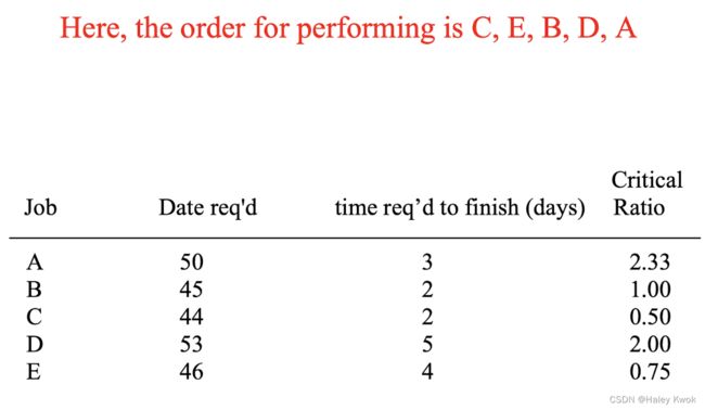
Critical Ratio (for reference)
Priority Rules
Supply Time (Time remaining until due date)/ Demand Time (Time needed to complete work)
The lower the ratio, the more critical the order is.
Chapter 9: Just-in-Time (JIT)/ Lean Manufacture
Toyota Production System
Much of Japan’s economic growth and prosperity has been attributed to the successful implementation of Just-In-Time (JIT)
1. Main Elements of JIT/Lean Production
Eliminate all types of waste, including carrying excessive levels of inventory and long lead times.
Eg: – produce or purchase items just in time to be used.
purchased materials -> fabricated parts -> sub-assemblies -> finished goods
The idea is to drive all queues toward zero in order to:
– minimize inventory investment,
– shorten production lead times,
– react faster to demand changes, and
– uncover any quality problems.
- A push system supply chain is one where projected demand determines what enters the process. (driven by demand)
- A pull system supply chain is one where products enter the supply chain when customer demand justifies it.
2. Inventory Hides Problems
- scraps
- unreliable suppliers
- capacity imbalance
Just-in-time production makes no allowances for contingencies.
– Every piece is expected to be correct when received.
– Every machine is expected to be available when needed to produce parts.
– Every delivery commitment is expected to be honored at the precise time it is scheduled.
3. Wastages
To make an advance in the process and enhance the added value.
Waste is anything that does not add value from the customer point of view
Eg.,
– Storage,
– inspection,
– delay,
– waiting in queues, and
– defective products
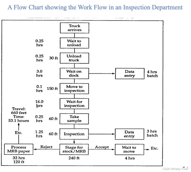
In the figure, it takes about 25 hours to have a good part accepted and about 32 hours to get a faulty part rejected.
Analysis can show that a great portion of the activities/time can be eliminated and thus the “actual working" time greatly reduced.
Categories of Waste
– Producing more than is necessary (over-producing) (excessive finished goods, by far the worst offense.)
– Unnecessary inventories (raw materials, component parts, sub-assemblies, WIP, finished goods)
– Operations and activities that do not add value to the product (non value added operations, over- processing)
– Production waiting time
– Temporary storage
– Unnecessary movement of man and materials.
– Producing defective parts and products
– An ideal condition for manufacturing is where there is no waste in machines, equipment and personnel.
4. Man-hour reduction
4.1 Elimination of waste
Knowing your workplace thoroughly well ,
Then achieve man-hour reduction by:
– Eliminate waste – Redistribute work – Reduce manpower
For example, reducing the waiting time, walking time by robotics
4.2 Redistribution of works
After eliminating non-value adding operations, can the net operations be redistributed?
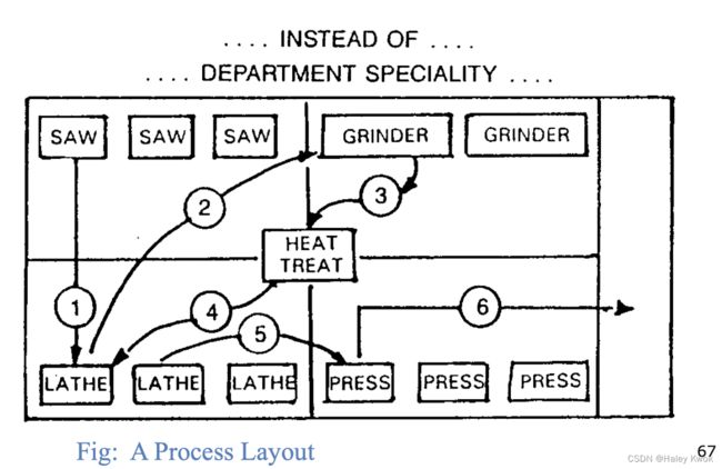
5. JIT Layout
In work re-distribution/combination, layout issues often arise: eg.,
– if an work area stands alone away from the rest,
– if a worker is surrounded by machines,
– if facilities are elongated, eg: the exit and entrance
may be far apart.
Even if workers have a desire to do more or to help each other, this is impossible.
How can we solve this problem?
Layout Tactics
– Build work cells for families of products – Minimize distance – Design minimum space for inventory – Build flexible or movable equipment – Cross train workers to add flexibilit
6. Leveling (Smoothing out) the Production System
The up and downs overtime in the workload generally lead to the creation of wastes.
Because
– The capacity of the workplace is often
adjusted to the peak work demand (and not
to its average)
Load smoothing in quantities and types
To achieve production equalization successfully, Leveling can be:
In quantities, AND
In the types of products to be processed.

Old schedule:
– AAAAAAAAA BBBBBBBBBBBBBBBBBBBBCCCCCCCC AAAAAAAAAA
New schedule:
– AABBB A B C B A C AA B CC A B A B C BB C AA C A B A
Because the lot size is small:
It is:
– Easier to change the production plan
– Increases the line’s flexibility in dealing with
– Reduce inventory.
• shorter order lead time • fluctuations in production quantities
required for each product.
7. Reduction of Machine Set-up Time
If the time for setting up is long, the economic production lot size is likely to remain larger.
This can lead to the waste arising from overproduction.
The only practical solution is:
–Shorten the setting up time required
An Approach for Set-up time Reduction
1) Separating the internal set-up from the external set-up activities.
Internal set-up activity: those that can only be performed while the machine is stopped.
External set-up activity: those that can be performed while the machine is running.
2) Further reducing internal set-up by
– reducing or eliminating the number of adjustments to the process to simplify the process, and – adding extra labour to the task when required.
8. Shorten the Lead time
Lead time can be defined as:
– the time elapsed from the time we start processing
materials into products to the time we receive payment for them (used by Toyota).
Eg., Operation lead time consists of:
– Queue – Setup – Run – Wait – Move
(Only “run” adds value to the product)
Ways to reduce lead time, eg.
– Combination of operations (eliminate all non-
value added times) – Reduced lot size (reduce queue time) – Level schedules (reduce queue time) – Work stations adjacent to each other (reduce
wait and move times)
9. Reduce Inventory
– Reduce lot sizes
– Reduce storage space for Inventory. (With reduced space, inventory must be in very small lot. Units are always moving because there is no storage space.)
– Use a pull system to move inventory
– Develop just-in-time delivery systems with suppliers
– Deliver directly to point of use
10. Zero Inventory as A Challenge
Of course it is practically impossible to have a zero inventory (zero defect), but that must be set as a goal.
If so, a manager will continue doing the following:
If you get to the one-half mark,
Reduce the remainder by half, and
Again reduce the remainder by half, and……
If this is done, the inventory can be significantly reduced.
11. The “Kanban” System
“Kanban” means signal.
It is usually a card or tag accompanying work-in-progress parts.
It serves as a work order.
– It gives at a glance information concerning
• what to produce,
• when to produce,
• in what quantity,
• by what means,
• the type of container to be used and
• how to transport it.
Kanban is a “pull” type of reorder system
ie: The authority to produce or supply comes from
downstream operations.
Two basic types of kanbans
The withdrawal kanban:
– An authorization to withdraw parts/materials from the preceding operation.
– It indicates the type and quantity of product which the next process should withdraw from the preceding process.
The production kanban:
– An authorization made to the preceding process to produce new parts/materials
– It specifies the type and quantity of product which the preceding process must produce.
Advantages of Kanban
– Allow only limited amount of faulty or delayed
material. – Problems are immediately evident. – Puts downward pressure on bad aspects of
inventory. – Standardized containers reduce weight, disposal costs, wasted space, and labour.
Determining the number of Kanbans
The no. of containers needed to support the user station
= average demand during the lead time plus some
safety stock, divided by the no. of units in one
container.
Number of Kanbans: Eg.,
Daily demand = 500 units
Production lead time (wait time + material handling time + processing time) = 2 days
Safety stock = 1/2 day
Container size = 250 units
Demand during lead time = 2 days x 500 units = 1,000
Number of kanbans = (1,000 + 250) / 250 = 5
12. JIT Partnership
JIT partnership exists
– when a supplier and purchaser work together to
remove waste and drive down cost.
13. Quality Circles
A quality circle is a group of volunteer employees who meet on a scheduled basis to
– Discuss their functions and the problems they’re
encountering
– Try to devise solutions to those problems and to propose those solutions to their management.
Circle members are taught:
– brain-storming techniques, – how to define a problem, – how to evaluate solutions, how to prepare flow
charts, – how to make a presentation to management so that
their proposals will sell,… etc.
14. Implementation of JIT
a) Commitment from Top Management
• Make sure that they know what changes will be required
and that they will provide the leadership to adopt the JIT approach.
• Prepare a plan of implementation.
b) Cooperation of the Work Force
• Strong leadership is needed on the factory floor to make
JIT work • Guarantee stable employment, engage in training, and
encourage participation in work improvement • Small-group improvement activities such as quality
circles should be used to get all employees involved in
problem solving • Begin training the work force to ensure job flexibility
c) Commence with the Final Assembly Line
• Schedule production to meet the demand only
• Reduce setup times until product models can be mixed
• Use standard containers for parts, and make them
readily accessible to the assembly line
d) Working backward from the Final Assembly Line • Reduce setup times and batch sizes of previous
operations to match the batch sizes needed in final assembly
• Remove inventory from the in-coming warehouse, and
locate inventory on the shop floor
e) Balance all previous Operations with production rates
on the Final Assembly
• This may require correction of capacity • Provide spare capacity in all areas so that if any work-
center falls behind, it will need some spare capacity in
order to catch up
f) Extend JIT to suppliers first, stabilize their delivery schedule and then ask for frequent deliveries.
• Remove the inventory needed to cover long lead-times
and variances. • Help vendors with quality assurance to meet your
specifications. • Negotiate long-term contracts with suppliers
5S
– Seiri
– Seiton
– Seisō
– Seiketsu Standardize
– Shitsuke Sustain, Self-discipline
Learn What 5S is and How it Applies to Any Industry https://www.youtube.com/watch?v=c0Q-xaYior0
Sort Straighten Sweep and Shine
Q: quantitive
Q23: qualitative