吴恩达老师机器学习课程练习2：逻辑回归python实现

a0.将所需数据放入当前工作目录

In [ ]:

!git clone https://github.com/fengdu78/Coursera-ML-AndrewNg-Notes.git
Cloning into 'Coursera-ML-AndrewNg-Notes'...
remote: Enumerating objects: 4762, done.
remote: Total 4762 (delta 0), reused 0 (delta 0), pack-reused 4762
Receiving objects: 100% (4762/4762), 643.40 MiB | 38.98 MiB/s, done.
Resolving deltas: 100% (1323/1323), done.
Checking out files: 100% (462/462), done.

In [ ]:

%cd /content/Coursera-ML-AndrewNg-Notes/code/ex2-logistic regression
/content/Coursera-ML-AndrewNg-Notes/code/ex2-logistic regression

1.线性回归

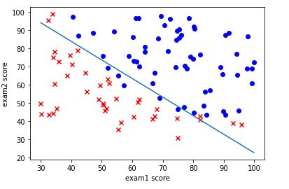
问题描述：应用逻辑回归模型预测一个学生是否能考上大学

数据集：之前同学两门课的成绩以及是否被允许入学

1.1可视化数据

In [ ]:

import numpy as np
import pandas as pd
import matplotlib.pyplot as plt

In [ ]:

data1 = pd.read_csv('./ex2data1.txt',names=['exam1','exam2','admitted'])
data1.describe()
data1.head()

Out[ ]:

	exam1	exam2	admitted
0	34.623660	78.024693	0
1	30.286711	43.894998	0
2	35.847409	72.902198	0
3	60.182599	86.308552	1
4	79.032736	75.344376	1

In [ ]:

for i in range(len(data1.exam1)):
  if data1.admitted[i] == 0:
    plt.scatter(data1.exam1[i], data1.exam2[i], marker='x', c='r')
  else:
    plt.scatter(data1.exam1[i], data1.exam2[i], marker='o',c='b')
plt.xlabel('exam1 score')
plt.ylabel('exam2 score')
plt.show

Out[ ]:

1.2实现

1.2.1sigmoid函数

In [ ]:

def smd(z):
  return 1 / (1 + np.exp(-z))

1.2.2代价函数和梯度

特别注意reshape()比T好用

In [ ]:

def cost(theta, x, y):
  m = len(y)
  inner = y * np.log(smd(x.dot(theta.reshape(3,1)))) + (1 - y) * np.log(1 - smd(x.dot(theta.reshape(3,1))))
  return -np.sum(inner) / m

data1.insert(0, 'Ones', 1)
x = data1.iloc[:,0:3]
y = data1.iloc[:,3:4]
#代价函数是应该是numpy矩阵，所以我们需要转换X和Y，然后才能使用它们。 我们还需要初始化theta。
x = np.array(x)
y = np.array(y)
theta = np.zeros((1,3))

cost(theta, x, y)

Out[ ]:

0.6931471805599453

In [ ]:

def gradient(theta, x, y):
  h = smd(x.dot(theta.reshape(3,1)))
  m = len(y)
  parameters = int(theta.size)
  g = np.zeros(parameters)


  for j in range(parameters):
    x_j = x[:,j].reshape((m,1))
    g[j] = np.sum((h - y) * x_j)/m
  return g

In [ ]:

gradient(theta, x, y)

Out[ ]:

array([ -0.1       , -12.00921659, -11.26284221])

1.2.3优化

In [ ]:

import scipy.optimize as opt
result = opt.fmin_tnc(func=cost, x0=theta, fprime=gradient, args=(x, y))
result

Out[ ]:

(array([-25.16131863,   0.20623159,   0.20147149]), 36, 0)

In [ ]:

cost(result[0], x, y)

Out[ ]:

0.20349770158947458

1.2.4评估

In [ ]:

for i in range(len(data1.exam1)):
  if data1.admitted[i] == 0:
    plt.scatter(data1.exam1[i], data1.exam2[i], marker='x', c='r')
  else:
    plt.scatter(data1.exam1[i], data1.exam2[i], marker='o',c='b')

X = np.linspace(data1.exam1.min(),data1.exam1.max(),100)
last_theta = result[0]
print(last_theta)
Y = (-last_theta[0] - last_theta[1]*X)/last_theta[2]
plt.plot(X, Y)

plt.xlabel('exam1 score')
plt.ylabel('exam2 score')
plt.show
[-25.16131863   0.20623159   0.20147149]

Out[ ]:

In [ ]:

def predict(theta, x):
  P = x.dot(theta.reshape(3,1))
  return [1 if x >= 0.5 else 0 for x in P]

In [ ]:

P = predict(result[0], x)
right = 0

for i in range(len(P)):
  if P[i] == y[i]:
    right += 1
acc = right*100/len(P)
print('准确率为{0}%'.format(acc))
准确率为89.0

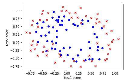
2.逻辑回归正则化

应用逻辑回归来判断一个芯片是否通过质检

2.1可视化数据

In [ ]:

data2 = pd.read_csv('./ex2data2.txt',names=['test1','test2','accepted'])
data2.head()

Out[ ]:

	test1	test2	accepted
0	0.051267	0.69956	1
1	-0.092742	0.68494	1
2	-0.213710	0.69225	1
3	-0.375000	0.50219	1
4	-0.513250	0.46564	1

In [ ]:

for i in range(len(data2.test1)):
  if data2.accepted[i] == 0:
    plt.scatter(data2.test1[i], data2.test2[i], marker='x', c='r')
  else:
    plt.scatter(data2.test1[i], data2.test2[i], marker='o',c='b')
plt.xlabel('test1 score')
plt.ylabel('test2 score')
plt.show

Out[ ]:

2.2实现

2.2.1 特征映射

In [ ]:

x1 = data2.test1
x2 = data2.test2
mapF = 6

for sum in range(mapF+1):
  for i in range(sum+1):
    data2['F' + str(i) + str(sum-i)] = np.power(x1, i) * np.power(x2, sum-i)

data2.head()

Out[ ]:

	test1	test2	accepted	F00	F01	F10	F02	F11	F20	F03	F12	F21	F30	F04	F13	F22	F31	F40	F05	F14	F23	F32	F41	F50	F06	F15	F24	F33	F42	F51	F60
0	0.051267	0.69956	1	1.0	0.69956	0.051267	0.489384	0.035864	0.002628	0.342354	0.025089	0.001839	0.000135	0.239497	0.017551	0.001286	0.000094	0.000007	0.167542	0.012278	0.000900	0.000066	0.000005	3.541519e-07	0.117206	0.008589	0.000629	0.000046	0.000003	2.477505e-07	1.815630e-08
1	-0.092742	0.68494	1	1.0	0.68494	-0.092742	0.469143	-0.063523	0.008601	0.321335	-0.043509	0.005891	-0.000798	0.220095	-0.029801	0.004035	-0.000546	0.000074	0.150752	-0.020412	0.002764	-0.000374	0.000051	-6.860919e-06	0.103256	-0.013981	0.001893	-0.000256	0.000035	-4.699318e-06	6.362953e-07
2	-0.213710	0.69225	1	1.0	0.69225	-0.213710	0.479210	-0.147941	0.045672	0.331733	-0.102412	0.031616	-0.009761	0.229642	-0.070895	0.021886	-0.006757	0.002086	0.158970	-0.049077	0.015151	-0.004677	0.001444	-4.457837e-04	0.110047	-0.033973	0.010488	-0.003238	0.001000	-3.085938e-04	9.526844e-05
3	-0.375000	0.50219	1	1.0	0.50219	-0.375000	0.252195	-0.188321	0.140625	0.126650	-0.094573	0.070620	-0.052734	0.063602	-0.047494	0.035465	-0.026483	0.019775	0.031940	-0.023851	0.017810	-0.013299	0.009931	-7.415771e-03	0.016040	-0.011978	0.008944	-0.006679	0.004987	-3.724126e-03	2.780914e-03
4	-0.513250	0.46564	1	1.0	0.46564	-0.513250	0.216821	-0.238990	0.263426	0.100960	-0.111283	0.122661	-0.135203	0.047011	-0.051818	0.057116	-0.062956	0.069393	0.021890	-0.024128	0.026596	-0.029315	0.032312	-3.561597e-02	0.010193	-0.011235	0.012384	-0.013650	0.015046	-1.658422e-02	1.827990e-02

2.2.2代价函数和梯度

In [ ]:

def cost2(theta, x, y, Lambda):
  m = len(y)
  n = np.size(theta)
  inner = y * np.log(smd(x.dot(theta.reshape(n,1)))) + (1 - y) * np.log(1 - smd(x.dot(theta.reshape(n,1))))
  first = -np.sum(inner) / m
  second = Lambda*np.sum(np.power(theta, 2))/m/2
  return first + second


x2 = data2.iloc[:,3:]
y2 = data2.iloc[:,2:3]
#代价函数是应该是numpy矩阵，所以我们需要转换X和Y，然后才能使用它们。 我们还需要初始化theta。
x2 = np.array(x)
y2 = np.array(y)
n = 28
theta2 = np.zeros((1,n))
Lambda = 1

cost2(theta2, x2, y2, Lambda)

Out[ ]:

0.6931471805599454

In [ ]:

def gradient2(theta, x, y, Lambda):
  n = np.size(theta)
  h = smd(x.dot(theta.reshape(n,1)))
  m = len(y)
  parameters = int(theta.size)
  g = np.zeros(parameters)
  theta = theta.reshape(1,n)


  for j in range(parameters):
    x_j = x[:,j].reshape((m,1))
    g[j] = np.sum((h - y) * x_j)/m + Lambda * theta[0,j]/m
  return g

gradient2(theta2, x2, y2, Lambda)

Out[ ]:

array([8.47457627e-03, 7.77711864e-05, 1.87880932e-02, 3.76648474e-02,
       1.15013308e-02, 5.03446395e-02, 2.34764889e-02, 8.19244468e-03,
       7.32393391e-03, 1.83559872e-02, 3.93028171e-02, 3.09593720e-03,
       1.28600503e-02, 2.23923907e-03, 3.93486234e-02, 3.10079849e-02,
       4.47629067e-03, 5.83822078e-03, 3.38643902e-03, 4.32983232e-03,
       1.99707467e-02, 3.87936363e-02, 1.37646175e-03, 7.26504316e-03,
       4.08503006e-04, 6.31570797e-03, 1.09740238e-03, 3.10312442e-02])

2.3优化

In [ ]:

result2 = opt.fmin_tnc(func=cost2, x0=theta, fprime=gradient2, args=(x2, y2, Lambda))
result2

Out[ ]:

(array([ 1.14201554,  1.16715861,  0.60123705, -1.26944057, -0.9156716 ,
        -1.87180883, -0.17391049, -0.34494285, -0.36850133,  0.12678647,
        -1.16320209, -0.26916597, -0.60631737, -0.04838602, -1.4237068 ,
        -0.46912463, -0.28708915, -0.28008563, -0.04305276, -0.20697497,
        -0.24269758, -0.93187605, -0.13795618, -0.32880531,  0.01716398,
        -0.29250738,  0.02904399, -1.0362975 ]), 26, 1)

2.4评估

绘制非线性决策边界就需要使用机器学习库了

In [ ]:

def predict(theta, x):
  n = np.size(theta)
  P = x.dot(theta.reshape(n,1))
  return [1 if x >= 0.5 else 0 for x in P]

P = predict(result2[0], x2)
right = 0

for i in range(len(P)):
  if P[i] == y[i]:
    right += 1
acc = right*100/len(P)
print('准确率为{0}%'.format(acc))
准确率为76.27118644067797%