机器学习（5）——决策树（预测隐形眼镜类型）

转载请注明作者和出处：https://blog.csdn.net/qq_28810395
Python版本： Python3.x
运行平台： Windows 10
IDE： Pycharm profession 2019
如有需要数据集或整个工程文件的可以关注cai_5158046回复决策树进行获取。

一、决策树简介

  处理分类问题，避免不料的就是对对象类别的决策，如同我们玩过的二十问题游戏 （出题的一方脑海中想象一个对象，答题的乙方进行提问，但只允许提问20个问题，初体的给予问题回答只能是对与错，答题人通过逐步推理分析，逐步缩小待猜测对象的范围），决策树的工作原理如同上述游戏过程，通过用户输入数据与反馈，逐步进行对象分类。
决策树的优缺点：

• 优点：计算复杂度不高，输出结果易于理解，对中间值的全是不敏感，可以处理不相关特征数据，一般适用与数值型与标称型数据类型。
• 缺点：可能会产生过度匹配问题。

二、决策树的构造

  总体来说，构造决策树分为三步：第一步进行信息论划分数据集的数学推演，第二步编写代码蒋理论应用到具体的数据集上，第三步编写代码构造决策树。
  对于算法，基本都是前有理论的推演，后有应用实践，在构造决策树进行数学推演中，我们首当其冲要解决的问题便是在众多特征中选择具有决定性的特征。

	不浮出水面是否可以生存	是否有脚蹼	属于鱼类
1	是	是	是
2	是	是	是
3	是	否	否
4	否	是	否
5	否	是	否

  如上表中，根据 “ 不浮出水面是否可以生存”、“是否有脚蹼” 两个特征进行分类，选 “ 不浮出水面是否可以生存” 进行分就比 “是否有脚蹼” 效果较好，所以对于特征的评估对划分数据集是及其重要的。下文就详细讨论如何选择最优特征进行数据集划分。

1.信息增益

  划分数据集最大的原则是：将无序的数据变得有序。
  在划分数据集之前我们要了解一些定义，对于划分数据集之前之后的变化我们称之为信息增益 ，信息增益的高低决定了选择划分数据集的特征选择是否最优，那信息增益如何计算呢？那我们就注定逃不开一个人——克劳德·香浓 （信息论之父），他提出了集合信息的度量方式——信息熵（熵），公式如下：

  详细理解请查看：https://www.cnblogs.com/loubin/p/11330576.html
  熵就是信息的期望值，我们需要计算所有类别所有可能包含的信息期望值，其中n那是分类的数目。
具体的Python实现程序如下：

#计算给定数据集的香农熵
from math import log
 
def calcShannonEnt(dataSet):
    numEntries = len(dataSet)  #
    labelCounts = {}
    # 以下五行为所有可能分类创建字典
    for featVec in dataSet:
        currentLabel = featVec[-1]  #提取最后一项做为标签
        if currentLabel not in labelCounts.keys():
            labelCounts[currentLabel] = 0
        labelCounts[currentLabel] += 1  # 书中有错
    # 0:{"yes":1} 1:{"yes":2}  2:{"no":1} 3:{"no":2} 4:{"no":3}
    shannonEnt = 0.0
    for key in labelCounts:
        prob = float(labelCounts[key]) / numEntries  # 计算概率
        # 以2为底求对数
        shannonEnt -= prob * log(prob,2) # 递减求和得熵

  下面我们进行测试，计算信息熵代码如下：

1. 创建测试数据集

#创建测试数据集
def createDataSet():
    dataSet = [[1, 1, 'yes'],
               [1, 1, 'yes'],
               [1, 0, 'no'],
               [0, 1, 'no'],
               [0, 1, 'no']]
    labels = ['no surfacing','flippers']
    #change to discrete values
    return dataSet, labels 

2. 进行测试

#进行测试
import trees

myDat,labels = trees.createDataSet()
print(myDat)
print('第1个',trees.calcShannonEnt(myDat))
myDat[0][-1]='maybe'
print(myDat)
print('第2个',trees.calcShannonEnt(myDat))

3. 结果

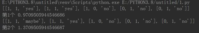
  从结果中可知，混合的数据越多，其信息熵就越高。

2.划分数据集

  计算信息熵，就是度量了数据集的无序程度，进行最优特征的选择要进行所有特征的信息熵计算，然后参照最优特征进行分类。

1. 对数据集进行划分的代码实现：

#划分数据集代码实现
def splitDataSet(dataSet,axis,value): # 三个输入参数：待划分的数据集、划分数据集的特征、需要返回的特征的值
    # 创建新的list对象
    retDataSet = []
    for featVec in dataSet:
        if featVec[axis] == value:  # dataSet[0]=0时执行以下操作
            # 以下三行抽取
            reducedFeatVec = featVec[:axis]   # featVec[:0]= [],即生成一个空列表
            reducedFeatVec.extend(featVec[axis + 1:]) # 添加index==1及后的元素 : 0/1/2 跳过,3:1,4:1
            retDataSet.append(reducedFeatVec) #整体作为元素添加 3:[[1,"no"]] , 4:[[1,"no"],[1,"no"]]
    return retDataSet

  然后将测算信息熵和划分数据集进行综合，找出最优的特征。

2. 寻找最优的特征

# 选择最好的数据集划分方式
def chooseBestFeatureToSplit(dataSet):
    numFeatures = len(dataSet[0]) - 1 # 去掉标签项
    baseEntropy = calcShannonEnt(dataSet) # 计算熵
    bestInfoGain = 0.0
    bestFeature = -1
    for i in range(numFeatures):
        # 以下两行创建唯一的分类标签列表
        featList = [example[i] for example in dataSet] # i=0:[1,1,1,0,0]  i=1:[1,1,0,1,1]
        uniqueVals = set(featList)  # i=0:{0,1}  i=1:{0,1}
        newEntropy = 0.0
        # 以下五行计算每种划分方式的信息熵
        for value in uniqueVals:
            subDataSet = splitDataSet(dataSet, i, value)
            prob = len(subDataSet)/float(len(dataSet))
            newEntropy += prob * calcShannonEnt(subDataSet)  # 注意这里是subDataSet 不是 dataSet
        infoGain = baseEntropy - newEntropy # 信息增益
        if (infoGain > bestInfoGain):
            # 计算最好的信息增益
            bestInfoGain = infoGain
            bestFeature = i
    return bestFeature

3. 测试：

myDat,labels = trees.createDataSet()
print('最优特征',trees.chooseBestFeatureToSplit(myDat))

4. 结果

  由结果看出，第0个特征是划分数据集的最优特征。对应上表的 “ 不浮出水面是否可以生存” 确实**相比 “是否有脚蹼” 划分最优。

3.递归构建决策树

  现在我们已经解决了第一个特征划分，因为现实情况肯定不止一个进行一次划分，所以存在两个分支以上的数据集划分，因此我们需要采用递归的方式进行数据集划分，直到遍历完所有划分数据集的属性。实现代码如下：

1. 创建决策树：

def createTree(dataSet,labels):
    classList = [example[-1] for example in dataSet]
    if classList.count(classList[0]) == len(classList): 
        return classList[0]#stop splitting when all of the classes are equal
    if len(dataSet[0]) == 1: #stop splitting when there are no more features in dataSet
        return majorityCnt(classList)
    bestFeat = chooseBestFeatureToSplit(dataSet)
    bestFeatLabel = labels[bestFeat]
    myTree = {bestFeatLabel:{}}
    del(labels[bestFeat])
    featValues = [example[bestFeat] for example in dataSet]
    uniqueVals = set(featValues)
    for value in uniqueVals:
        subLabels = labels[:]       #copy all of labels, so trees don't mess up existing labels
        myTree[bestFeatLabel][value] = createTree(splitDataSet(dataSet, bestFeat, value),subLabels)
    return myTree              

2. 测试：

myDat,labels = trees.createDataSet()
myTree = trees.createTree(myDat,labels )
print(myTree)

3. 结果

  在这我们已经完成了决策树的构造。下面我将进行决策树可视化的讲解。

三、利用Matplotlib进行决策树可视化显示

  由于上述结果为字典形式，对于决策树字典的表示形式不容易被理解，而且直接绘制图形也比较困难，所以我们利用Matplotlib进行决策树的可视化显示。
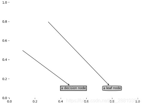
在决策树中常有的关系就是树形的指向关系，所以我们采用箭头直线指向目标框的方式进行表示。

1.代码实现

import matplotlib.pyplot as plt

decisionNode = dict(boxstyle="sawtooth", fc="0.8")
leafNode = dict(boxstyle="round4", fc="0.8")
arrow_args = dict(arrowstyle="<-")
def plotNode(nodeTxt, centerPt, parentPt, nodeType):
    createPlot.ax1.annotate(nodeTxt, xy=parentPt,  xycoords='axes fraction',
             xytext=centerPt, textcoords='axes fraction',
             va="center", ha="center", bbox=nodeType, arrowprops=arrow_args )
def createPlot_0():
   fig = plt.figure(1, facecolor='white')
   fig.clf()
   createPlot.ax1 = plt.subplot(111, frameon=False) #ticks for demo puropses
   plotNode('a decision node', (0.5, 0.1), (0.1, 0.5), decisionNode)
   plotNode('a leaf node', (0.8, 0.1), (0.3, 0.8), leafNode)
   plt.show()

2.测试与结果显示

myDat,labels = trees.createDataSet()
treePlotter.createPlot_0()

3.绘制注解树

  构造一棵完整的注解树，首先要对树的叶节点数目和树的层数进行获取，也就是对字典数据进行处理。

1. 获取叶节点的数目和树层数

#获取叶节点的数目
def getNumLeafs(myTree):
    numLeafs = 0
    firstStr = myTree.keys()[0]
    secondDict = myTree[firstStr]
    for key in secondDict.keys():
        if type(secondDict[key]).__name__=='dict':#test to see if the nodes are dictonaires, if not they are leaf nodes
            numLeafs += getNumLeafs(secondDict[key])
        else:   numLeafs +=1
    return numLeafs
#获取树层数
def getTreeDepth(myTree):
    maxDepth = 0
    firstStr = myTree.keys()[0]
    secondDict = myTree[firstStr]
    for key in secondDict.keys():
        if type(secondDict[key]).__name__=='dict':#test to see if the nodes are dictonaires, if not they are leaf nodes
            thisDepth = 1 + getTreeDepth(secondDict[key])
        else:   thisDepth = 1
        if thisDepth > maxDepth: maxDepth = thisDepth
    return maxDepth

2. 绘制注解树相关函数代码

#在父子节点之间填充文本信息
def plotMidText(cntrPt, parentPt, txtString):
    xMid = (parentPt[0]-cntrPt[0])/2.0 + cntrPt[0]
    yMid = (parentPt[1]-cntrPt[1])/2.0 + cntrPt[1]
    createPlot.ax1.text(xMid, yMid, txtString, va="center", ha="center", rotation=30)
#计算宽与高
def plotTree(myTree, parentPt, nodeTxt):#if the first key tells you what feat was split on
    numLeafs = getNumLeafs(myTree)  #this determines the x width of this tree
    depth = getTreeDepth(myTree)
    firstStr = myTree.keys()[0]     #the text label for this node should be this
    cntrPt = (plotTree.xOff + (1.0 + float(numLeafs))/2.0/plotTree.totalW, plotTree.yOff)
    plotMidText(cntrPt, parentPt, nodeTxt)
    plotNode(firstStr, cntrPt, parentPt, decisionNode)
    secondDict = myTree[firstStr]
    plotTree.yOff = plotTree.yOff - 1.0/plotTree.totalD
    for key in secondDict.keys():
        if type(secondDict[key]).__name__=='dict':#test to see if the nodes are dictonaires, if not they are leaf nodes   
            plotTree(secondDict[key],cntrPt,str(key))        #recursion
        else:   #it's a leaf node print the leaf node
            plotTree.xOff = plotTree.xOff + 1.0/plotTree.totalW
            plotNode(secondDict[key], (plotTree.xOff, plotTree.yOff), cntrPt, leafNode)
            plotMidText((plotTree.xOff, plotTree.yOff), cntrPt, str(key))
    plotTree.yOff = plotTree.yOff + 1.0/plotTree.totalD
#if you do get a dictonary you know it's a tree, and the first element will be another dict
#
def createPlot(inTree):
    fig = plt.figure(1, facecolor='white')
    fig.clf()
    axprops = dict(xticks=[], yticks=[])
    createPlot.ax1 = plt.subplot(111, frameon=False, **axprops)    #no ticks
    #createPlot.ax1 = plt.subplot(111, frameon=False) #ticks for demo puropses 
    plotTree.totalW = float(getNumLeafs(inTree))
    plotTree.totalD = float(getTreeDepth(inTree))
    plotTree.xOff = -0.5/plotTree.totalW; plotTree.yOff = 1.0;
    plotTree(inTree, (0.5,1.0), '')
    plt.show()

3. 结果

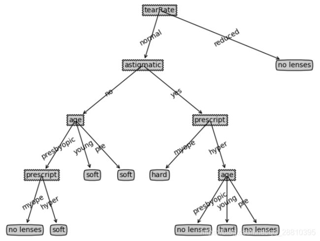
四、利用决策树预测隐形眼镜实例

1.数据数据集并分类代码

# 6预测隐形眼镜
fr = open('lenses.txt')
lenses = [inst.strip().split('\t') for inst in fr.readlines()]
lensesLabels = ['age', 'prescript', 'astigmatic', 'tearRate']
lensestree=trees.createTree(lenses, lensesLabels)
print(lensestree)
treePlotter.createPlot(lensestree)

2.结果

{'tearRate': {'normal': {'astigmatic': {'no': {'age': {'presbyopic': {'prescript': 
{'myope': 'no lenses', 'hyper': 'soft'}}, 'young': 'soft', 'pre': 'soft'}}, 'yes': 
{'prescript': {'myope': 'hard', 'hyper': {'age': {'presbyopic': 'no lenses', 
'young':'hard', 'pre': 'no lenses'}}}}}}, 'reduced': 'no lenses'}}

五、参考信息

机器学习实战