matlab实现TSAI标定及其误差分析
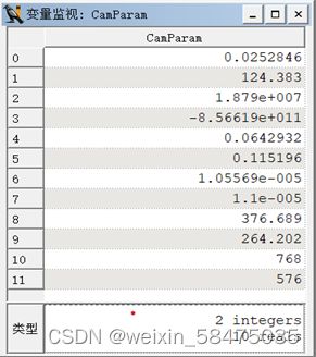
1.结果截图

2.结果讨论
用FASI标定的结果得到的结果图如图三所示,用HALCON得到的标定结果如图四所示。由于是用手机进行拍照,得到的相机内部参数不全,于是本次实验结果仅讨论焦距。手机拍照时的真实焦距为25mm,比较两次实验结果的相对误差可得,FASI与真实焦距的相对误差为7.228%,HALCON与真实焦距的相对误差为11.384%。就焦距这一项数据而言,FASI的准确率更高。
3.食用方法
将提取到的特征点写入ImageCoordinate.txt文件,将特征点所对应的真实世界坐标写入WordCoordinate.txt,运行testData.m即可。
4.代码
专业课老师给的代码
testData.m
clc
clear all
x=load('WordCoordinate.txt');
X=load('ImageCoordinate.txt');
Xf=X(:,1); %图像横坐标,表示像素
Yf=X(:,2);%图像纵坐标,表示像素
xw=x(:,1);
yw=x(:,2);
[M,N]=size(x);
zw=zeros(M,1);
Ncx=1;%可理解为平面像素的采样频率,一般设置为1
Nfx=1;
Cx=640; %Cx,Cy是像平面中心像素位置,即U0,V0
Cy=512;
dx=0.0052;%每个像素的物理尺寸
dy=0.0052;
sx=1;%相当于误差项,也设置为1
[R, T, f, k1] = Tsai(Xf, Yf, xw, yw, zw, Ncx, Nfx, dx, dy, Cx, Cy, sx);
a=atan(-R(2,3)/R(3,3));
a1=a*180/pi;
c=atan(-R(1,2)/R(1,1));
c1=c*180/pi;
q=cos(c);
b=atan(R(1,3)*q/R(1,1));
b1=b*180/pi;
Tsai.m
% [R, T, f, k1] = Tsai (Xf, Yf, xw, yw, zw, Ncx, Nfx, dx, dy, Cx, Cy, sx)
%
% **********************************************************************************************
% ******* Calibrating a Camera Using a Monoview Coplanar Set of Points *******
% **********************************************************************************************
% 6/2004 Simon Wan
% simonwan@hit.edu.cn
%
% Note: Xf, Yf, xw, yw, zw are all column vectors
%
% (xw, yw, zw) is the 3D coordinate of the object point P in the 3D world coordinate system
% (x, y, z) is ths 3D coordinate of the object point P in the 3D camera coordinate system
% (X, Y) is the image coordinate system centered at Oi where is the intersection of the optical center axis z and the front plane
% (Xu, Yu) is the image coordinate of (x, y, z) if a perfect pinhole
% camera model is used(利用相机坐标表示的图像坐标)
% Xu = f * x / z (4a)
% Yu = f * y / z (4b)
% (Xd, Yd) is the actual image coordinate which differs from (Xu, Yu)
% due to lens distortion实际的图像坐标(加了畸变)
% (Xf, Yf) is the coordinate used in the computer, is the number of
% pixels for the discrete image in the frame memory(像素坐标)
% R is the 3*3 rotation matrix
% = [r1, r2, r3; r4, r5, r6; r7, r8, r9]; (2)
% [x, y, z]' = R * [xw, yw, zw]' + T (1)
% T is the translation vector
% = [Tx, Ty, Tz]' (3)
% f is the effective focal length 是有效的焦距
% Dx = Xd*( k1*r^2 + k2*r^4 + ... ) P327
% Xd+Dx=Xu (5a)
% Dy = Yd*( k1*r^2 + k2*r^4 + ... ) P327
% Yd+Dy=Yu (5b)
% r = (Xd^2 + Yd^2)^(0.5) P327
% k1 is the distortion coeffient
% Xf = sx * dxp^(-1) * Xd + Cx (6a)
% Yf = dy^(-1) * Yd + Cy (6b)
% dxp = dx * Ncx / Nfx (6d)
% dx is the center to center distance between adjacent sensor elements in X (scan line) diretion是X(扫描线)方向上相邻传感器元件之间的中心距离
% dy is the center to center distance between adjacent CCD sensor in the Y direction是相邻CCD传感器在Y方向上的中心距离
% Ncx is the number of sensor elements in the X direction是X方向上的传感器元件的数量,平面像素的采样频率
% Nfx is the number of pixels in a line as sampled by the computer是计算机采样的行中像素数,表明平面像素的采样频率
% sx is the uncertainty image scale factor是不确定性图像比例因子,相当于误差项,也设置为1
% X = (Xd * Nfx) / (dx * Ncx) P328
% X = Xf - Cx P328
% Y = Yf - Cy P328
% sx^(-1)*dxp*X + sz^(-1)*dxp*X*k1*r^2 = f*x/z (7a)
% dxp*Y + dy*Y*k1*r^2 = f*y/z (7b)
% r = ( ( sx^(-1)*dxp*X )^2 + (dx*Y)^2 )^(0.5)
% sx^(-1)*dxp*X + sx^(-1)*dxp*X*k1*r^2 = f*(r1*xw + r2*yw + r3*zw +
% Tx) / (r7*xw + r8*yw + r9*zw +Tz) (8a)
% dy*Y + dy*Y*k1*r^2 = f*(r1*xw + r2*yw + r3*zw +
% Tx) / (r7*xw + r8*yw + r9*zw +Tz) (8b)
% Since the calibration points are on a common plane, the (xw, yw, zw) coordinate system can be chosen such that zw=0 and the
% corigin is not lose to the center of the view or y axis of the camera coordinate system. Since the (xw, yw, zw) is user-defined
% and the origin is arbitrary, it is no problem setting the origin of (xw, yw, zw) to be out of the field of view and not close
% to the y axis. the purpose for the latter is to make sure that Ty is not exactly zero.
%
% REF: "A versatile camera calibration technique for high-accuracy 3D machine
% vision metrology using off-the-shelf TV cameras and lens"
% R.Y. Tsai, IEEE Trans R&A RA-3, No.4, Aug 1987, pp 323-344.
%
function [R, T, f, k1] = Tsai(Xf, Yf, xw, yw, zw, Ncx, Nfx, dx, dy, Cx, Cy, sx)
% Stage 1 --- Compute 3D Orientation, Position (x and y):
% a) Compute the distored image coordinates (Xd, Yd) Procedure:
dxp = dx * Ncx / Nfx;
X = Xf - Cx;
Y = Yf - Cy;
Xd=sx^(-1)*dxp*(Xf-Cx);
Yd=dy*(Yf-Cy);
% b) Compute the five unknowns Ty^(-1)*r1, Ty^(-1)*r2, Ty^(-1)*Tx, Ty^(-1)*r4, Ty^(-1)*r5
% r1p=Ty^(-1)*r1;
% r2p=Ty^(-1)*r2;
% Txp=Ty^(-1)*Tx;
% r4p=Ty^(-1)*r4;
% r5p=Ty^(-1)*r5;
A=[Yd.*xw Yd.*yw Yd -Xd.*xw -Xd.*yw];
B=Xd;
C=A\B;
r1p=C(1);
r2p=C(2);
Txp=C(3);
r4p=C(4);
r5p=C(5);
clear A B C;
% c) Compute (r1,...,r9,Tx,Ty) from (Ty^(-1)*r1, Ty^(-1)*r2, Ty^(-1)*Tx, Ty^(-1)*r4, Ty^(-1)*r5):
% 1) Compute |Ty| from (Ty^(-1)*r1, Ty^(-1)*r2, Ty^(-1)*Tx, Ty^(-1)*r4, Ty^(-1)*r5):
C=[r1p, r2p; r4p, r5p];
Sr=r1p^2 + r2p^2 + r4p^2 + r5p^2;
if rank(C)==2
Ty2=( Sr - (Sr^2-4*(r1p*r5p-r4p*r2p)^2)^(0.5) )/(2*(r1p*r5p-r4p*r2p)^2);
else
z = C(abs(C) > 0);
Ty2 = 1.0 / (z(1)^2 + z(2)^2);
end
Ty = sqrt(Ty2);
clear C Sr Ty2 z
% 2) Determine the sign of Ty:
[ymax i] = max(Xd.^2 + Yd.^2);
r1 = r1p*Ty;
r2 = r2p*Ty;
r4 = r4p*Ty;
r5 = r5p*Ty;
Tx = Txp*Ty;
x = r1*xw(i) + r2*yw(i) + Tx;
y = r4*xw(i) + r5*yw(i) + Ty;
% if (sign(x) == sign(Xf(i))) & (sign(y) == sign(Yf(i))),
if (sign(x) == sign(X(i))) && (sign(y) == sign(Y(i))),
Ty = Ty;
else
Ty = -Ty;
end
clear ymax i x y
% 3) Compute the 3D rotation matrix R, or r1, r2,...,r9
r1 = r1p*Ty;
r2 = r2p*Ty;
r4 = r4p*Ty;
r5 = r5p*Ty;
Tx = Txp*Ty;
s = -sign(r1*r4 + r2*r5);
R=[r1, r2, (1-r1^2-r2^2)^(0.5); r4, r5, s*(1-r4^2-r5^2)^(0.5)];
R = [R(1:2,:); cross(R(1,:), R(2,:))];
r7 = R(3,1);
r8 = R(3,2);
r9 = R(3,3);
y = r4*xw+r5*yw+Ty;
w = r7*xw+r8*yw;
z = [y -dy*Y] \ [dy*(w.*Y)];
f = z(1);
if f < 0
R(1,3) = -R(1,3);
R(2,3) = -R(2,3);
R(3,1) = -R(3,1);
R(3,2) = -R(3,2);
end
r3 = R(1,3);
r6 = R(2,3);
r7 = R(3,1);
r8 = R(3,2);
clear s y w z
% 2) Stage 2 --- Compute Effective Focal Length, Distortion Coefficients, and z Position:
% d) Compute an approximation of f and Tz by ignoring lens distortion:
y = r4*xw+r5*yw+Ty;
w = r7*xw+r8*yw;
z = [y -dy*Y] \ [dy*(w.*Y)];
f = z(1);
Tz = z(2);
% Compute the exactly solution for f, Tz, k1:
params_const = [r4 r5 r6 r7 r8 r9 dx dy sx Ty];
params = [f, Tz, 0]; % add initial guess for k1
[x,fval,exitflag,output] = fminsearch( @Tsai_8b, params, [], params_const, xw, yw, zw, X, Y);
f = x(1);
Tz = x(2);
k1 = x(3);
T=[Tx, Ty, Tz]';
% fval the value of the objective function fun at the solution x.
fval
% exitflag that describes the exit condition of fminsearch
% >0 Indicates that the function converged to a solution x.
% 0 Indicates that the maximum number of function evaluations was exceeded.
% <0 Indicates that the function did not converge to a solution.
exitflag
% output that contains information about the optimization
% output.algorithmThe algorithm used
% output.funcCountThe number of function evaluations
% output.iterationsThe number of iterations taken
output
Tsai_8b.m
% f = Tsai_8b(params, params_const, xw, yw, zw, X, Y)
%
% **********************************************************************************************
% ******* Calibrating a Camera Using a Monoview Coplanar Set of Points *******
% **********************************************************************************************
% 6/2004 Simon Wan
% simonwan@hit.edu.cn
%
% Note: This is not called directly but as a function handle from the "fminsearch "
%
function f = Tsai_8b(params, params_const, xw, yw, zw, X, Y)
% unpack the params
f = params(1);
Tz = params(2);
k1 = params(3);
% unpack the params_const
r4 = params_const(1);
r5 = params_const(2);
r6 = params_const(3);
r7 = params_const(4);
r8 = params_const(5);
r9 = params_const(6);
dx = params_const(7);
dy = params_const(8);
sx = params_const(9);
Ty = params_const(10);
rsq = (dx*X).^2 + (dy*Y).^2;
res = (dy*Y).*(1+k1*rsq).*(r7*xw+r8*yw+r9*zw+Tz) - f*(r4*xw+r5*yw+r6*zw+Ty);
f = norm(res, 2);
5.结果:
运行代码后,结果及其误差分析会在当前目录下生成txt文件。