图像梯度算子——Sobel/scharr/Laplacian

1.sobel算子

sobel算子可以计算图像梯度，计算图像梯度的作用是提取边界。

（1）X方向的梯度

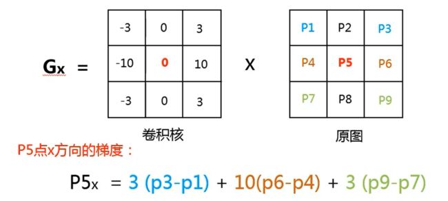
以3x3的卷积核计算sobel算子为例：

图中左边就是计算水平梯度时的卷积核，简单来说就是右边减左边，权重由卷积核规定。

含义：当目标（P5点）右左两列差别特别大的时候，目标点的值会很大，说明该点为边界。

（2）Y方向的梯度

上图是计算垂直方向梯度的卷积核，如果在垂直方向上存在有较大的差值就说明存在有水平边界。

（3）注意&总结

a.水平梯度运算提取垂直方向的边界，垂直方向的梯度运算得到水平方向的边界。

b.Opencv默认的是截断的操作，即小于0按0算，大于255按255算。这样计算得到的图像可能会被削半，不合适，最好对于小于0的取绝对值，大于255的可按255算（最大的极差了）。

（4）总梯度

总梯度：

 简化梯度：

（5）函数介绍

cv.Sobel(	
            src, 
            ddepth, 
            dx, 
            dy[, dst[, ksize[, scale[, delta[, borderType]]]]]	
) 

->	dst

Parameters

src	input image.
dst	output image of the same size and the same number of channels as src .
ddepth	output image depth, see combinations; in the case of 8-bit input images it will result in truncated derivatives.
dx	order of the derivative x.
dy	order of the derivative y.
ksize	size of the extended Sobel kernel; it must be 1, 3, 5, or 7.
scale	optional scale factor for the computed derivative values; by default, no scaling is applied (see getDerivKernels for details).
delta	optional delta value that is added to the results prior to storing them in dst.
borderType	pixel extrapolation method, see BorderTypes. BORDER_WRAP is not supported.

 参考：OpenCV: Image Filtering

代码测试：

import cv2
import numpy as np
# 获取照片路径
path=r"C:\Users\Nobody\Desktop\Hand.JPG"
# 读取照片
img=cv2.imread(path,0)
# 显示照片
# cv2.imshow('image',img)
# 缩放
img1=cv2.resize(img,None,fx=0.4,fy=0.4)
# cv2.imshow('img1', img1)

# 计算X方向的梯度
sobelx=cv2.Sobel(img1,cv2.CV_64F,1,0,ksize=3)
# 将复数转化为整数【绝对值函数】
sobelx=cv2.convertScaleAbs(sobelx)
# cv2.imshow('sobelx',sobelx)

# 计算y方向的梯度
sobely=cv2.Sobel(img1,cv2.CV_64F,0,1,ksize=3)
# 将复数转化为整数【绝对值函数】
sobely=cv2.convertScaleAbs(sobely)
# cv2.imshow('sobely',sobely)

# 融合
sobelxy1=cv2.addWeighted(sobelx,0.5,sobely,0.5,0)
# cv2.imshow('sobelxy1',sobelxy1)

# 直接计算融合的X和Y梯度
sobelxy2=cv2.Sobel(img1,cv2.CV_64F,1,1,ksize=3)
# 将复数转化为整数【绝对值函数】
sobelxy2=cv2.convertScaleAbs(sobelxy2)
# cv2.imshow('sobelxy2',sobelxy2)
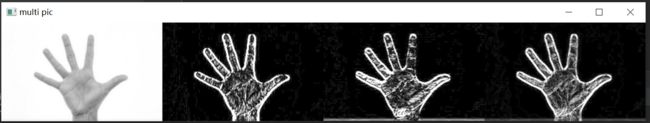
imgs = np.hstack([img1, sobelx,sobely,sobelxy1,sobelxy2])
cv2.imshow('multi pic',imgs)
cv2.waitKey()

 结果输出：

总结：

融合计算的X和Y梯度，比直接计算X和Y的梯度，效果要好。

2.scharr算子

scharr与sobel算子思想一样，只是卷积核的系数不同，scharr算子提取边界也更加灵敏，能提取到更细小的边界，但请注意，越是灵敏就越是可能误判。

（1）X方向的梯度

 

 

 （2）Y方向的梯度

 （3）函数介绍

cv.Scharr(	
            src, 
            ddepth, 
            dx, 
            dy[, dst[, scale[, delta[, borderType]]]]	
) 

->	dst

 Parameters

src	input image.
dst	output image of the same size and the same number of channels as src.
ddepth	output image depth, see combinations
dx	order of the derivative x.
dy	order of the derivative y.
scale	optional scale factor for the computed derivative values; by default, no scaling is applied (see getDerivKernels for details).
delta	optional delta value that is added to the results prior to storing them in dst.
borderType	pixel extrapolation method, see BorderTypes. BORDER_WRAP is not supported.

注意：

dx和dy均大于等于0/dx+dy==1(只能先计算x和y，然后再进行融合)

无卷积核参数，默认是3*3

参考：OpenCV: Image Filtering

（4）测试代码

import cv2
import numpy as np
# 获取照片路径
path=r"C:\Users\Nobody\Desktop\Hand.JPG"
# 读取照片
img=cv2.imread(path,0)
# 显示照片
# cv2.imshow('image',img)
# 缩放
img1=cv2.resize(img,None,fx=0.4,fy=0.4)
# cv2.imshow('img1', img1)

# 计算X方向的梯度
scharrx=cv2.Scharr(img1,cv2.CV_64F,1,0)
# 将复数转化为整数【绝对值函数】
scharrx=cv2.convertScaleAbs(scharrx)
# cv2.imshow('scharrx',scharrx)

# 计算y方向的梯度
scharry=cv2.Scharr(img1,cv2.CV_64F,0,1)
# 将复数转化为整数【绝对值函数】
scharry=cv2.convertScaleAbs(scharry)
# cv2.imshow('scharry',scharry)

# 融合
scharrxy=cv2.addWeighted(scharrx,0.5,scharry,0.5,0)
# cv2.imshow('scharrxy',scharrxy)

imgs = np.hstack([img1, scharrx,scharry,scharrxy])
cv2.imshow('multi pic',imgs)
cv2.waitKey()

结果输出：

 

3.Laplacian算子

Laplacian算子也是用来计算图像梯度的，作用也是提取边界。它与上面两种算子的不同是：
sobel算子和scharr算子一般先算一个水平梯度，再算一个垂直方向梯度，然后把两个结果按照0.5的权重进行图像融合以得到完整的边界。

但Laplacian算子则不同，它本身就是一个二阶的算子，它的运算规则就是在水平方向运算两次，垂直方向运算两次，两个结果相叠加替换中心点（锚点）的像素值（灰度值）。

拉普拉斯算子类似于二阶sobel导数。实际上，在OpenCV中通过调用sobel算子来计算拉普拉斯算子。使用的公式为：

（1）梯度计算

（2）函数介绍

cv.Laplacian(	
                src, 
                ddepth[, dst[, ksize[, scale[, delta[, borderType]]]]]	
) 

->	dst

Parameters

src	Source image.
dst	Destination image of the same size and the same number of channels as src .
ddepth	Desired depth of the destination image.
ksize	Aperture size used to compute the second-derivative filters. See getDerivKernels for details. The size must be positive and odd.
scale	Optional scale factor for the computed Laplacian values. By default, no scaling is applied. See getDerivKernels for details.
delta	Optional delta value that is added to the results prior to storing them in dst .
borderType	Pixel extrapolation method, see BorderTypes. BORDER_WRAP is not supported.

 参考：

OpenCV: Image Filtering

（3）代码测试

import cv2
import numpy as np
# 获取照片路径
path=r"C:\Users\Nobody\Desktop\Hand.JPG"
# 读取照片
img=cv2.imread(path,0)
# 显示照片
# cv2.imshow('image',img)
# 缩放
img1=cv2.resize(img,None,fx=0.4,fy=0.4)
# cv2.imshow('img1', img1)
new_img=cv2.Laplacian(img1,cv2.CV_64F)
new_img=cv2.convertScaleAbs(new_img)
imgs=np.hstack([img1,new_img])
cv2.imshow('multi pic',imgs)
cv2.waitKey()

cv2.waitKey()

结果输出：

 总结：

拉普拉斯对噪声点比较敏感，一般不单独使用