基于scikit-learn的鸢尾花分类实例

基于scikit-learn的鸢尾花分类实例

代码参考书籍：Python机器学习基础教程. Andreas C.muller, Sarah Guido著（张亮 译）. 北京：人民邮电出版社，2018.1(2019.6重印)

实现环境

System：Ubuntu server 20.04 (Jupyter notebook)
GPU：GeForce GTX 1080Ti（2块）
Driver Version: 450.36.06
CUDA Version: 11.0
Python Version: 3 .8.5
TensorFlow Version：2.4.1
————————————————
版权声明：本文为CSDN博主「技术无极限」的原创文章，遵循CC 4.0 BY-SA版权协议，转载请附上原文出处链接及本声明。
原文链接：https://blog.csdn.net/bilvqing108/article/details/113706050

根据已知品种的鸢尾花测量数据，构建机器学习模型，这是一个监督学习的问题。
在多个选项中预测其中一个结果，这个一个分类问题。
分类的每一个可能输出叫做类别。

![sepal_petal](images/iris_petal_sepal.png)

1. 初始数据

#从scikit-learn的datasets载入数据。这是一个公开数据集。
from sklearn.datasets import load_iris
iris_dataset = load_iris()    #载入的数据保存在iris_dataset中

查看数据集，做到心中有数，…

#得到的数据集是一个Bunch对象，它和字典dict非常相似，因此，可以查看它的关键字，以掌握数据集的内容
print("Keys of iris_dataset:\n", iris_dataset.keys())   #查看数据集关键字

输出：
Keys of iris_dataset:
dict_keys([‘data’, ‘target’, ‘frame’, ‘target_names’, ‘DESCR’, ‘feature_names’, ‘filename’])

print(iris_dataset['DESCR'][:193] + "\n...")    #数据集的说明

输出：
… _iris_dataset:
Iris plants dataset
--------------------Data Set Characteristics:
:Number of Instances: 150 (50 in each of three classes)
:Number of Attributes: 4 numeric, pre…

print("Target names:", iris_dataset['target_names'])    #目标名称，是我们要预测的花的品种。它是一个字符串数组

输出：
Target names: [‘setosa’ ‘versicolor’ ‘virginica’]

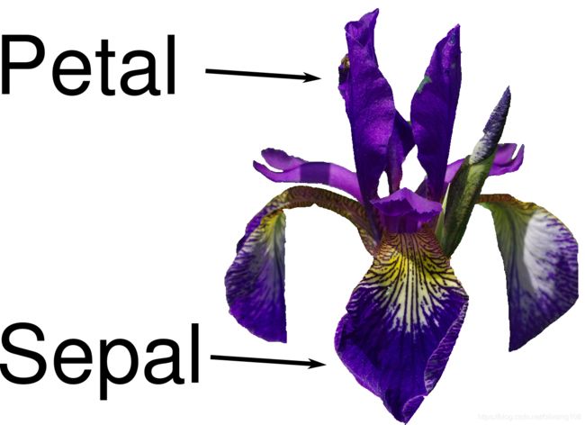
print("Feature names:\n", iris_dataset['feature_names'])    #特征属性名称，也是一个字符串数组

输出：
Feature names:
[‘sepal length (cm)’, ‘sepal width (cm)’, ‘petal length (cm)’, ‘petal width (cm)’]

print("Type of data:", type(iris_dataset['data']))    #特征值 ，是一个Numpy的（150,4）二维数组。type()查看数据的类型

输出：
Type of data:

print("Shape of data:", iris_dataset['data'].shape)    #.shape查看数据的维度

输出：
Shape of data: (150, 4)

print("First five rows of data:\n", iris_dataset['data'][:5])    #预览前5个样本的特征值

输出：
First five rows of data:
[[5.1 3.5 1.4 0.2]
[4.9 3. 1.4 0.2]
[4.7 3.2 1.3 0.2]
[4.6 3.1 1.5 0.2]
[5. 3.6 1.4 0.2]]

print("Type of target:", type(iris_dataset['target']))    #标签值 ，是一个Numpy的（150,）一维数组。

输出：
Type of target:

print("Shape of target:", iris_dataset['target'].shape)

输出：
Shape of target: (150,)

print("Target:\n", iris_dataset['target'])    #预览所有标签值

输出：
Target:
[0 0 0 0 0 0 0 0 0 0 0 0 0 0 0 0 0 0 0 0 0 0 0 0 0 0 0 0 0 0 0 0 0 0 0 0 0
0 0 0 0 0 0 0 0 0 0 0 0 0 1 1 1 1 1 1 1 1 1 1 1 1 1 1 1 1 1 1 1 1 1 1 1 1
1 1 1 1 1 1 1 1 1 1 1 1 1 1 1 1 1 1 1 1 1 1 1 1 1 1 2 2 2 2 2 2 2 2 2 2 2
2 2 2 2 2 2 2 2 2 2 2 2 2 2 2 2 2 2 2 2 2 2 2 2 2 2 2 2 2 2 2 2 2 2 2 2 2
2 2]

2. 衡量模型是否成功：训练数据与测试数据

构建模型后，在需要使用模型进行预测前，需要验证模型是否有效，就需要有验证模型的数据集。
数据分割：把数据分为训练集和测试集
scikit-learn的train_test_split函数可以打乱数据集并进行拆分。这个函数将75%的行数据及对应标签（样本）作为训练集，剩下的25%作为测试集。
数据的打乱是利用伪随机数生成器实现的，需要指定参数random_state指定随机数生成器的种子。它为0时，不管运行多少次，函数的输出固定不变。

from sklearn.model_selection import train_test_split    #从scikit-learn中加载train_test_split()
X_train, X_test, y_train, y_test = train_test_split(
    iris_dataset['data'], iris_dataset['target'], random_state=0)     #实现数据的拆分

print("X_train shape:", X_train.shape)     #查看分割后的数据集大小，注意，特征数组是二维的，但标签数组是一维的
print("y_train shape:", y_train.shape)

输出：
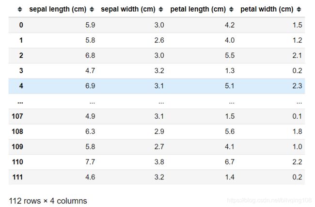
X_train shape: (112, 4)
y_train shape: (112,)

print("X_test shape:", X_test.shape)
print("y_test shape:", y_test.shape)

输出：
X_test shape: (38, 4)
y_test shape: (38,)

3. 第一要事：观察数据

# create dataframe from data in X_train
# label the columns using the strings in iris_dataset.feature_names
#构建pandas数据框架（数据结构）
iris_dataframe = pd.DataFrame(X_train, columns=iris_dataset.feature_names)
#DataFrame()中，第一个参数是存放在DataFrame里的数据，第二个参数index就是之前说的行名(这里省略了)，第三个参数columns是之前说的列名。参见：https://pandas.pydata.org/pandas-docs/stable/reference/api/pandas.DataFrame.html
#其中后两个参数可以使用list输入，但是注意，这个list的长度要和DataFrame的大小匹配，不然会报错。
# create a scatter matrix from the dataframe, color by y_train  散点矩阵图，颜色有y_train标签决定
#函数scatter_matrix()的说明见如下官网。
#https://pandas.pydata.org/pandas-docs/stable/reference/api/pandas.plotting.scatter_matrix.html
#pandas.plotting.scatter_matrix(frame, alpha=0.5, figsize=None, ax=None, grid=False, diagonal='hist', marker='.', density_kwds=None, hist_kwds=None, range_padding=0.05, **kwargs)
#cmap 颜色表
pd.plotting.scatter_matrix(iris_dataframe, c=y_train, figsize=(15, 15),
                           marker='o', hist_kwds={'bins': 20}, s=60,
                           alpha=.8, cmap=mglearn.cm3)

输出：
array([[,
,
,
],
[,
,
,
],
[,
,
,
],
[,
,
,
]],
dtype=object)

display(iris_dataframe)    #列表显示训练数据

4. 构建第一个模型：K近邻算法

K近邻算法：是最简单的机器学习算法。构建模型只需要保存训练数据集即可。
要对新的数据样本做出预测，算法会在训练数据中找到最近的数据点，也就是它的“最近邻”。
然后根据最近邻的K个数据点中，标签数最多的类别作为预测结果。

rom sklearn.neighbors import KNeighborsClassifier   #加载K近邻分类器函数
knn = KNeighborsClassifier(n_neighbors=1)    #取近邻数k=1,也就是，最靠近样本标签值就是它的预测值。

knn.fit(X_train, y_train)    #训练模型，对应k近邻算法，其实就是保存数据

输出：
KNeighborsClassifier(n_neighbors=1)

5. 做出预测

X_new = np.array([[5, 2.9, 1, 0.2]])    #要预测的数据样本，注意要转换为二维Numpy数组的一行，（1,4）一行四列
print("X_new.shape:", X_new.shape)

输出：
X_new.shape: (1, 4)

prediction = knn.predict(X_new)     #利用predict()函数实现预测
print("Prediction:", prediction)
print("Predicted target name:",
       iris_dataset['target_names'][prediction])    #输出预测值与预测类别

输出：
Prediction: [0]
Predicted target name: [‘setosa’]

6. 评估模型

上面的预测结果是否可靠，还需要对模型进行评估后，才能做出判断。

y_pred = knn.predict(X_test)     #对所有的测试集数据集进行预测，再跟原来的标签进行对比，计算出测试精度。
print("Test set predictions:\n", y_pred)

输出：
Test set predictions:
[2 1 0 2 0 2 0 1 1 1 2 1 1 1 1 0 1 1 0 0 2 1 0 0 2 0 0 1 1 0 2 1 0 2 2 1 0
2]

print("Test set score: {:.2f}".format(np.mean(y_pred == y_test)))    #利用Numpy的mean()函数求预测精度。

输出：
Test set score: 0.97

print("Test set score: {:.2f}".format(knn.score(X_test, y_test)))    #也可以利用knn对象的score()评分函数，来计算模型的精度

输出：
Test set score: 0.97

示例结束！