吴恩达机器学习课程笔记+代码实现(4)Python实现单变量线性回归和梯度下降(Programming Exercise 1.1)
Programming Exercise 1: Linear Regression
Python版本3.6
编译环境:anaconda Jupyter Notebook
链接:ex1data1.txt、ex1data2.txt 和编程作业ex1.pdf(实验指导书)
提取码:i7co
1 单变量线性回归(Linear regression with one variable)
本章课程笔记部分见:单变量线性回归和梯度下降
1.1数据可视化(Plotting the Data)
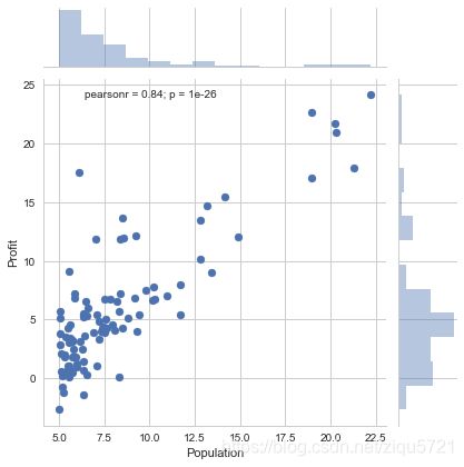
The file ex1data1.txt contains the dataset for our linear regression problem. The first column is the population of a city and the second column is the profit of a food truck in that city. A negative value for profit indicates a loss.
%matplotlib inline
#IPython的内置magic函数,可以省掉plt.show(),在其他IDE中是不会支持的
import numpy as np
import pandas as pd
import matplotlib as mpl
import matplotlib.pyplot as plt
from matplotlib.colors import LogNorm
from mpl_toolkits.mplot3d import axes3d, Axes3D
import seaborn as sns
sns.set(style="whitegrid",color_codes=True)
df = pd.read_csv("ex1data1.txt",header=None,names=["Population","Profit"])
df.head()#查看数据前5项
| Population | Profit | |
|---|---|---|
| 0 | 6.1101 | 17.5920 |
| 1 | 5.5277 | 9.1302 |
| 2 | 8.5186 | 13.6620 |
| 3 | 7.0032 | 11.8540 |
| 4 | 5.8598 | 6.8233 |
df.describe()#查看数据相关统计
| Population | Profit | |
|---|---|---|
| count | 97.000000 | 97.000000 |
| mean | 8.159800 | 5.839135 |
| std | 3.869884 | 5.510262 |
| min | 5.026900 | -2.680700 |
| 25% | 5.707700 | 1.986900 |
| 50% | 6.589400 | 4.562300 |
| 75% | 8.578100 | 7.046700 |
| max | 22.203000 | 24.147000 |
df.info()#查看数据DataFrame
RangeIndex: 97 entries, 0 to 96
Data columns (total 2 columns):
Population    97 non-null float64
Profit        97 non-null float64
dtypes: float64(2)
memory usage: 1.6 KB
将数据用散点图表示
sns.jointplot(x="Population",y="Profit",data=df)
1.2 梯度下降
现在利用梯度下降找出拟合数据集的线性回归参数θ
线性回归的目标是最小化参数θ为特征函数的代价函数
J ( θ ) = 1 2 m ∑ i = 1 m ( h θ ( x ( i ) ) − y ( i ) ) 2 J\left( \theta \right)=\frac{1}{2m}\sum\limits_{i=1}^{m}{{{\left( {{h}_{\theta }}\left( {{x}^{(i)}} \right)-{{y}^{(i)}} \right)}^{2}}} J(θ)=2m1i=1∑m(hθ(x(i))−y(i))2
而: h θ ( x ) = θ T X = θ 0 x 0 + θ 1 x 1 + θ 2 x 2 + . . . + θ n x n {{h}_{\theta }}\left( x \right)={{\theta }^{T}}X={{\theta }_{0}}{{x}_{0}}+{{\theta }_{1}}{{x}_{1}}+{{\theta }_{2}}{{x}_{2}}+...+{{\theta }_{n}}{{x}_{n}} hθ(x)=θTX=θ0x0+θ1x1+θ2x2+...+θnxn
本案例中是单变量线性回归,假设
h θ ( x ) = θ T X = θ 0 + θ 1 x 1 {{h}_{\theta }}\left( x \right)={{\theta }^{T}}X={{\theta }_{0}}+{{\theta }_{1}}{{x}_{1}} hθ(x)=θTX=θ0+θ1x1
#计算代价函数
def computeCost(X,Y,theta):
    h = X.dot(theta.T)
    cost = np.power((h - Y),2)
    j = np.sum(cost)/(2 * len(X))
    return j
由于 h θ ( x ) = θ T X = θ 0 + θ 1 x 1 {{h}_{\theta }}\left( x \right)={{\theta }^{T}}X={{\theta }_{0}}+{{\theta }_{1}}{{x}_{1}} hθ(x)=θTX=θ0+θ1x1
故为实现向量化相乘的操作,数据集中增加一列数值为1的数据,即 X 0 = 1 X_{0}=1 X0=1
df.insert(0,"x_0",1)
| x_0 | Population | Profit | |
|---|---|---|---|
| 0 | 1 | 6.1101 | 17.5920 |
| 1 | 1 | 5.5277 | 9.1302 |
| 2 | 1 | 8.5186 | 13.6620 |
| 3 | 1 | 7.0032 | 11.8540 |
| 4 | 1 | 5.8598 | 6.8233 |
将数据集中抽离输入X与结果Y
X = df.loc[:,"x_0":"Population"]
X.head()
| x_0 | Population | |
|---|---|---|
| 0 | 1 | 6.1101 |
| 1 | 1 | 5.5277 |
| 2 | 1 | 8.5186 |
| 3 | 1 | 7.0032 |
| 4 | 1 | 5.8598 |
Y = df.iloc[:,2:3]
Y.head()
| Profit | |
|---|---|
| 0 | 17.5920 |
| 1 | 9.1302 |
| 2 | 13.6620 |
| 3 | 11.8540 |
| 4 | 6.8233 |
将X与Y转化矩阵
X = np.matrix(X.values)
Y = np.matrix(Y.values)
初始化参数θ矩阵
theta = np.matrix(np.zeros((1, 2)))
matrix([[0., 0.]])
print(computeCost(X,Y,theta))##计算一下初始时theta为0的代价函数
32.072733877455676
批量梯度下降更新参数θ: θ j : = θ j − α ∂ ∂ θ j J ( θ ) {{\theta }_{j}}:={{\theta }_{j}}-\alpha \frac{\partial }{\partial {{\theta }_{j}}}J\left( \theta \right) θj:=θj−α∂θj∂J(θ)
∂ ∂ θ j J ( θ 0 , θ 1 ) = ∂ ∂ θ j 1 2 m ∑ i = 1 m ( h θ ( x ( i ) ) − y ( i ) ) 2 \frac{\partial }{\partial {{\theta }_{j}}}J({{\theta }_{0}},{{\theta }_{1}})=\frac{\partial }{\partial {{\theta }_{j}}}\frac{1}{2m}{{\sum\limits_{i=1}^{m}{\left( {{h}_{\theta }}({{x}^{(i)}})-{{y}^{(i)}} \right)}}^{2}} ∂θj∂J(θ0,θ1)=∂θj∂2m1i=1∑m(hθ(x(i))−y(i))2
j = 0 j=0 j=0 时: ∂ ∂ θ 0 J ( θ 0 , θ 1 ) = 1 m ∑ i = 1 m ( h θ ( x ( i ) ) − y ( i ) ) \frac{\partial }{\partial {{\theta }_{0}}}J({{\theta }_{0}},{{\theta }_{1}})=\frac{1}{m}{{\sum\limits_{i=1}^{m}{\left( {{h}_{\theta }}({{x}^{(i)}})-{{y}^{(i)}} \right)}}} ∂θ0∂J(θ0,θ1)=m1i=1∑m(hθ(x(i))−y(i))
j = 1 j=1 j=1 时: ∂ ∂ θ 1 J ( θ 0 , θ 1 ) = 1 m ∑ i = 1 m ( ( h θ ( x ( i ) ) − y ( i ) ) ⋅ x ( i ) ) \frac{\partial }{\partial {{\theta }_{1}}}J({{\theta }_{0}},{{\theta }_{1}})=\frac{1}{m}\sum\limits_{i=1}^{m}{\left( \left( {{h}_{\theta }}({{x}^{(i)}})-{{y}^{(i)}} \right)\cdot {{x}^{(i)}} \right)} ∂θ1∂J(θ0,θ1)=m1i=1∑m((hθ(x(i))−y(i))⋅x(i))
则算法改写成:
Repeat {
θ 0 : = θ 0 − a 1 m ∑ i = 1 m ( h θ ( x ( i ) ) − y ( i ) ) {\theta_{0}}:={\theta_{0}}-a\frac{1}{m}\sum\limits_{i=1}^{m}{ \left({{h}_{\theta }}({{x}^{(i)}})-{{y}^{(i)}} \right)} θ0:=θ0−am1i=1∑m(hθ(x(i))−y(i))
θ 1 : = θ 1 − a 1 m ∑ i = 1 m ( ( h θ ( x ( i ) ) − y ( i ) ) ⋅ x ( i ) ) {\theta_{1}}:={\theta_{1}}-a\frac{1}{m}\sum\limits_{i=1}^{m}{\left( \left({{h}_{\theta }}({{x}^{(i)}})-{{y}^{(i)}} \right)\cdot {{x}^{(i)}} \right)} θ1:=θ1−am1i=1∑m((hθ(x(i))−y(i))⋅x(i))
}
def gradientDescent(X,Y,theta,alpha,n):
    temp = np.matrix(np.zeros(theta.shape))
    s = int(theta.ravel().shape[1])#得到theta矩阵个数
    j_theta = np.zeros(n)
    for i in range(n):
        cost = (X * theta.T) - Y
        for j in range(s):
            term = np.multiply(cost,X[:,j])
            temp[0,j] = theta[0,j] - ((alpha / len(X)) * np.sum(term))
        theta = temp
        j_theta[i] = computeCost(X,Y,theta)
    return theta ,j_theta
alpha = 0.01
n = 1000
th,cost = gradientDescent(X,Y,theta,alpha,n)
th
matrix([[-3.24140214, 1.1272942 ]])
线性回归函数可视化
a = th[0,1]
b = th[0,0]
fig, ax = plt.subplots(figsize=(10,6))
ax.scatter(df.Population, df.Profit, label="Training data")
ax.plot(df.Population, df.Population*a + b, label="Prediction",color = "red")
plt.legend(loc=2)
ax.set_xlabel('Population')
ax.set_ylabel('Profit')

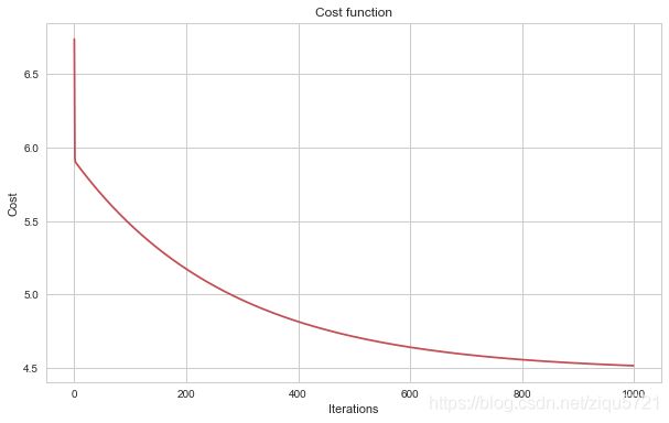
代价函数可视化
与迭代次数之间的关系
fig, ax = plt.subplots(figsize=(10,6))
ax.plot(np.arange(n), cost, 'r')
ax.set_xlabel('Iterations')
ax.set_ylabel('Cost')
ax.set_title('Cost function')
Text(0.5,1,'Cost function')
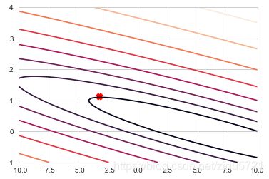
与参数之间的关系
theta0_vals = np.linspace(-10, 10, 100)  #参数1的取值
theta1_vals = np.linspace(-1, 4, 100)    #参数2的取值


xs, ys = np.meshgrid(theta0_vals, theta1_vals)   #生成网格
J_vals = np.zeros(xs.shape)

for i in range(0, theta0_vals.size):
    for j in range(0, theta1_vals.size):
        t = np.array([theta0_vals[i], theta1_vals[j]])
       # t = t.T
        J_vals[i][j] = computeCost(X, Y, t)    #计算每个网格点的代价函数值

J_vals = np.transpose(J_vals)

fig1 = plt.figure(1)      #绘制3d图形
ax = fig1.gca(projection='3d')
ax.plot_surface(xs, ys, J_vals)
plt.xlabel(r'$\theta_0$')
plt.ylabel(r'$\theta_1$')

#绘制等高线图 相当于3d图形的投影
plt.figure(2)
lvls = np.logspace(-5, 5, 50)
plt.contour(xs, ys, J_vals, levels=lvls, norm=LogNorm())
plt.scatter(b,a, marker="x",color="red",linewidth=5)

参考资料:吴恩达机器学习课程编程作业实验指导书ex1.pdf;