Advances in Graph Neural Networks笔记2：Fundamental Graph Neural Networks

诸神缄默不语-个人CSDN博文目录

本书网址：https://link.springer.com/book/10.1007/978-3-031-16174-2
本文是本书第二章的学习笔记。

我们学校没买这书，但是谷歌学术给我推文献时给出了一个能免登录直接上的地址，下次就不一定好使了，所以我火速阅读原文并做笔记。
因此常识性内容我就略去不写了，可以看我以前写过的详细笔记。
阅读体验是，内容概括比较全面，但是写得很含混，就跟通用大学教材一样……可以略读一遍来作为引导，但是以本书为教材的指望大概难以实现。不如cs224w和浙大GNN课程。

GNN中最具有代表性的图卷积神经网络将卷积操作从网格（grid）数据泛化到图（graph）数据上，分成以图信号处理角度切入的谱域（spectral based）和以信息传播角度切入的空域（spatial based）。GCN是这两种图卷积网络之间的过渡方法，近期空域方法更火（因为有效且灵活）。
本章将先从谱域视角介绍GCN，再介绍空域的GCN变体（包括inductive框架GraphSAGE、用注意力机制聚合邻居的GAT、对异质图做semantic-level attention的HAN）

（本书参考文献部分的序号与正文不匹配，我也懒得一一去查了，所以就不写参考文献了）

1. 谱域GCN

CNN在视觉任务中成功的原因之一：卷积层能分层级抽取图像高维特征，通过学习一组固定尺寸的可训练局部滤波器（fixed-size trainable localized filters）提升表现能力。

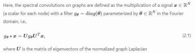
图数据非欧，从谱域视角，基于图傅里叶变换定义图卷积，可以通过两个傅里叶变换后的图信号的乘积的逆傅里叶变换来计算：
图谱域卷积的定义：图信号与滤波器（以 $\theta \in {\mathbb{R}}^N$ 对参数角矩阵）在傅里叶域的乘积：

借助normalized graph Laplacian的特征向量来求解。可以通过切比雪夫多项式来简化：

GCN模型对谱域图卷积操作做出了简化：将切比雪夫多项式卷积操作减到一阶（K=1），并近似${\lambda }_{max}\approx 2$：

继续进行简化：

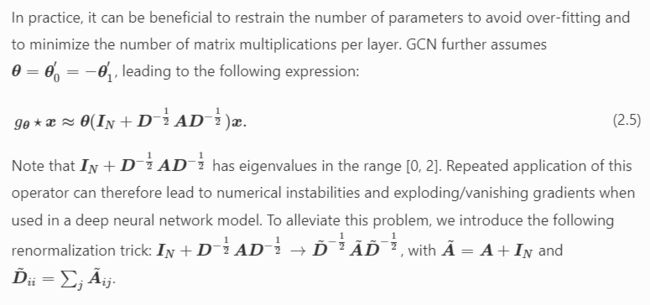
得到泛化后的图卷积表达式：

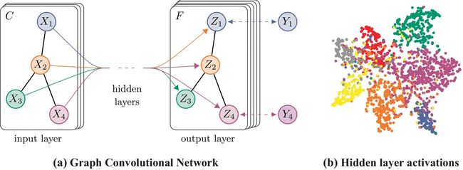
左图：半监督学习任务图解
右图：两层GCN在Cora数据集上用5%标签实现半监督任务学习，其隐藏层的t-SNE可视化。颜色表示文档类别

通过表达式实现学习任务：

2. inductive GCN→GraphSAGE

抽样、聚合新节点局部邻居特征，实现inductive节点表征。

可以mini-batch训练。

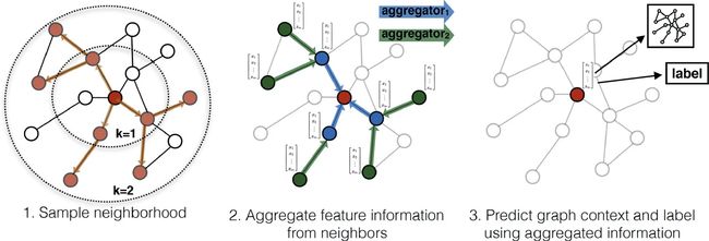
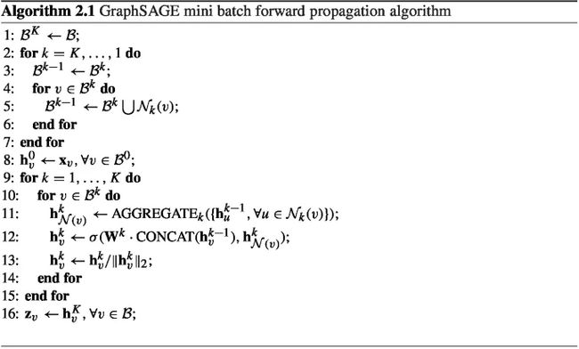
Neighborhood Sampler
GCN的输入：固定大小的整个图
GraphSAGE：对mini-batch中的每个节点选择固定数量的邻居

Neighborhood Aggregator

1. Mean aggregator（近于GCN）
   $$\begin{array}{r}{\text{h}}_v^k\leftarrow \sigma (\text{W}\cdot \text{MEAN}(\{{\text{h}}_v^{k-1}\}\bigcup \{{\text{h}}_u^{k-1},\forall u\in \mathcal{N}(v)\})).\end{array}$$
2. LSTM aggregator：将节点邻居随机打乱
3. Pooling aggregator
   $$\begin{array}{r}\text{A}GGREGAT{E}_k^{pool}=\text{m}ax(\{\sigma ({\text{W}}_{pool}{\text{h}}_u^k+\text{b}),\forall u\in \mathcal{N}(v)\}).\end{array}$$

3. GAT

在GCN基础上添加attention机制，加权求和

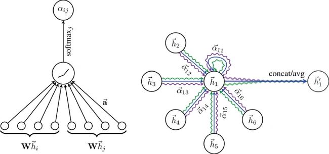
左图：注意力
右图：多头（3）注意力机制

attention机制总之就是在最终结果之上增加了一个权重计算机制，具体内容有时间和能力的话我再专门写个博客讲一下。

将节点对进行线性转换后，用单层前馈神经网络$\mathbf{a}$得到标量attention coefficients（节点$j$对节点$i$的重要性）：
$$\begin{array}{r}{e}_{ij}=\text{attn}(\text{W}{\text{h}}_i,\text{W}{\text{h}}_j)\end{array}$$

masked注意力机制 - 仅用邻居节点计算注意力：
$$\begin{array}{rl}& {\alpha }_{ij}={\text{softmax}}_j(e_{ij})=\frac{\text{exp}(e_{ij})}{{\sum }_{k\in {\mathcal{N}}_i}\text{exp}(e_{ik})}\\ & {\alpha }_{ij}=\frac{\text{exp}(\text{LeakyReLU}({\text{a}}^T[\text{W}{\text{h}}_i\Vert \text{W}{\text{h}}_j]))}{{\sum }_{k\in {\mathcal{N}}_i}\text{exp}(\text{LeakyReLU}({\text{a}}^T[\text{W}{\text{h}}_i\Vert \text{W}{\text{h}}_k]))}\end{array}$$

加权求和：
$$\begin{array}{r}{\text{h}}_i=\sigma \left(\sum _{j\in {\mathcal{N}}_i}{\alpha }_{ij}\text{W}{\text{h}}_j\right)\end{array}$$

多头注意力机制：
$$\begin{array}{r}{\text{h}}_i={\Vert }_{k=1}^K\sigma \left(\sum _{j\in {\mathcal{N}}_i}{\alpha }_{ij}^k{\text{W}}^k{\text{h}}_j\right)\end{array}$$

最后一层：
$$\begin{array}{r}{\text{h}}_i=\sigma \left(\frac{1}{K}\sum _{k=1}^K\sum _{j\in {\mathcal{N}}_i}{\alpha }_{ij}^k{\text{W}}^k{\text{h}}_j\right)\end{array}$$

attention可以提供更强的模型表示能力，一定的可解释性，而且可做inductive范式。

4. HAN

Heterogeneous graph Attention Network (HAN)
将GCN扩展到异质图上：官方的说法是通过学习node-level attention and semantic-level attention来学习节点和metapaths的重要性，其实就是先对每种metapath聚合所有邻居、然后再聚合所有metapath得到的表征（用了两种不同的注意力机制）、最终得到目标节点的表征。

meta-path
meta-path-based neighbors

先用node attention对每个metapath选择重要的meta-path-based neighbors，得到semantic-specific node embedding；再用semantic attention选择重要的metapath

Node-level Attention
先将各种节点映射到对应类型的隐空间，然后计算每个metapath下邻居的注意力机制，用多头注意力机制稳定训练过程：
$$\begin{array}{rl}& {\text{h}}_i^{\prime }={\text{M}}_{{\varphi }_i}\cdot {\text{h}}_i\\ & e_{ij}^{\Phi }=at{t}_{node}({\text{h}}_i^{\prime },{\text{h}}_j^{\prime };\Phi )\\ & {\alpha }_{ij}^{\Phi }=softma{x}_j(e_{ij}^{\Phi })=\frac{\exp (\sigma ({\text{a}}_{\Phi }^{\text{T}}\cdot [{\text{h}}_i^{\prime }\Vert {\text{h}}_j^{\prime }]))}{{\sum }_{k\in {\mathcal{N}}_i^{\Phi }}\exp (\sigma ({\text{a}}_{\Phi }^{\text{T}}\cdot [{\text{h}}_i^{\prime }\Vert {\text{h}}_k^{\prime }]))}\\ & {\text{z}}_i^{\Phi }=\sigma (\sum _{j\in {\mathcal{N}}_i^{\Phi }}{\alpha }_{ij}^{\Phi }\cdot {\text{h}}_j^{\prime })\\ & {\text{z}}_i^{\Phi }=\stackrel{K}{\underset{k=1}{\Vert }}\sigma (\sum _{j\in {\mathcal{N}}_i^{\Phi }}{\alpha }_{ij}^{\Phi }\cdot {\text{h}}_j^{\prime })\end{array}$$

Semantic-level Aggregation
直接对每个metapath的所有节点上的表征通过MLP后，tanh激活、线性转换、加总、归一化（除以节点数），然后对所有这些结果做softmax归一化。
$$\begin{array}{r}{w}^{\Phi }=\frac{1}{|\mathcal{V}|}\sum _{v\in \mathcal{V}}{\text{q}}^T\cdot tanh(\text{W}\cdot {\text{z}}_v^{\Phi }+\text{b}),\end{array}$$

用得到的权重计算最终的节点表征：
$$\begin{array}{r}{\text{z}}_v=\sum _{\Phi \in \{{\Phi }_1,\dots ,{\Phi }_P\}}{\beta }^{\Phi }\cdot {\text{z}}_v^{\Phi }.\end{array}$$

5. GCN启发出的其他GNN

recurrent graph neural networks
graph autoencoders

6. 其他推荐阅读材料

直接建议左转我的其他博文。

1. 《Advances in Graph Neural Networks》第1~2章读书笔记：这个里面还写了我没法看的第一章的相关内容。yysy，我觉得这篇写得比本书要好点，但都有一个很严重的问题，就是过于简略，就像论文里的preliminary，说了个寂寞，懂的人不用看，不懂的人看不懂。