OpenCV_06 图像平滑：图像噪声+图像平滑+滤波

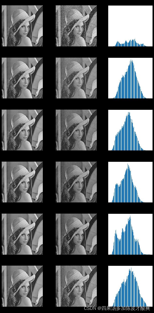
1 图像噪声

由于图像采集、处理、传输等过程不可避免的会受到噪声的污染，妨碍人们对图像理解及分析处理。常见的图像噪声有高斯噪声、椒盐噪声等。

1.1 椒盐噪声

椒盐噪声也称为脉冲噪声，是图像中经常见到的一种噪声，它是一种随机出现的白点或者黑点，可能是亮的区域有黑色像素或是在暗的区域有白色像素（或是两者皆有）。椒盐噪声的成因可能是影像讯号受到突如其来的强烈干扰而产生、类比数位转换器或位元传输错误等。例如失效的感应器导致像素值为最小值，饱和的感应器导致像素值为最大值。
椒盐噪声的概率密度函数为：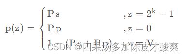

1.2 高斯噪声

高斯噪声是指噪声密度函数服从高斯分布的一类噪声。由于高斯噪声在空间和频域中数学上的易处理性，这种噪声(也称为正态噪声)模型经常被用于实践中。高斯随机变量z的概率密度函数由下式给出：

$$p(z)=\frac{1}{\sqrt{2\pi }\sigma }{e}^{\frac{-(z-\mu {)}^2}{2{\sigma }^2}}$$

其中$z$表示灰度值，$\mu$表示$z$的平均值或期望值，$\sigma$表示$z$的标准差。标准差的平方${\sigma }^2$​​称为$z$的方差。高斯函数的曲线如图所示:

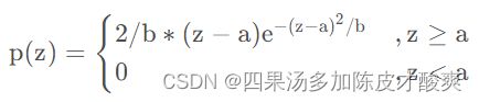
1.3 瑞利噪声

瑞利噪声的概率密度函数为

1.4 伽马噪声

伽马噪声又称爱尔兰噪声，其概率密度函数为

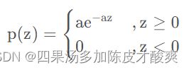
1.5 指数噪声

指数噪声的概率密度函数为

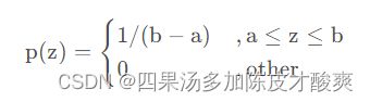
1.6 均匀噪声

均匀噪声的概率密度函数为

示例：

"""
高斯噪声
"""
import cv2
import matplotlib.pyplot as plt
import numpy as np


img = cv2.imread("./src_data/lena.jpg", 0)

# 椒盐噪声
ps, pp = 0.05, 0.02
mask = np.random.choice((0, 0.5, 1), size=img.shape[:2], p=[pp, (1 - ps - pp), ps])
imgChoiceNoise = img.copy()
imgChoiceNoise[mask == 1] = 255
imgChoiceNoise[mask == 0] = 0

# 高斯噪声
mu, sigma = 0.0, 20.0
noiseGause = np.random.normal(mu, sigma, img.shape)
imgGaussNoise = img + noiseGause
imgGaussNoise = np.uint8(cv2.normalize(imgGaussNoise, None, 0, 255, cv2.NORM_MINMAX))  # 归一化为 [0,255]

# 瑞利噪声
a = 30.0
noiseRayleigh = np.random.rayleigh(a, size=img.shape)
imgRayleighNoise = img + noiseRayleigh
imgRayleighNoise = np.uint8(cv2.normalize(imgRayleighNoise, None, 0, 255, cv2.NORM_MINMAX))  # 归一化为 [0,255]

# 伽马噪声
a, b = 10.0, 2.5
noiseGamma = np.random.gamma(shape=b, scale=a, size=img.shape)
imgGammaNoise = img + noiseGamma
imgGammaNoise = np.uint8(cv2.normalize(imgGammaNoise, None, 0, 255, cv2.NORM_MINMAX))  # 归一化为 [0,255]

# 指数噪声
a = 10.0
noiseExponent = np.random.exponential(scale=a, size=img.shape)
imgExponentNoise = img + noiseExponent
imgExponentNoise = np.uint8(cv2.normalize(imgExponentNoise, None, 0, 255, cv2.NORM_MINMAX))  # 归一化为 [0,255]

# 均匀噪声
mean, sigma = 10, 100
a = 2 * mean - np.sqrt(12 * sigma)  # a = -14.64
b = 2 * mean + np.sqrt(12 * sigma)  # b = 54.64
noiseUniform = np.random.uniform(a, b, img.shape)
imgUniformNoise = img + noiseUniform
imgUniformNoise = np.uint8(cv2.normalize(imgUniformNoise, None, 0, 255, cv2.NORM_MINMAX))  # 归一化为 [0,255]

plt.figure(figsize=(9, 18))
# 椒盐噪声
plt.subplot(631), plt.title("Origin"), plt.axis('off')
plt.imshow(img, 'gray', vmin=0, vmax=255)
plt.subplot(632), plt.title("ChoiceNoise"), plt.axis('off')
plt.imshow(imgChoiceNoise, 'gray')
plt.subplot(633), plt.title("ChoiceNoise Hist")
histNP, bins = np.histogram(imgChoiceNoise.flatten(), bins=255, range=[0, 255], density=True)
plt.bar(bins[:-1], histNP[:])
# 高斯噪声
plt.subplot(634), plt.title("Origin"), plt.axis('off')
plt.imshow(img, 'gray', vmin=0, vmax=255)
plt.subplot(635), plt.title("GaussNoise"), plt.axis('off')
plt.imshow(imgGaussNoise,'gray')
plt.subplot(636), plt.title('GaussNoise Hist')
histNP, bins = np.histogram(imgGaussNoise.flatten(), bins=255, range=[0, 255], density=True)
plt.bar(bins[:-1], histNP[:])
# 瑞利噪声
plt.subplot(6,3,7), plt.title("Origin"), plt.axis('off')
plt.imshow(img, 'gray', vmin=0, vmax=255)
plt.subplot(6,3,8), plt.title("RayleighNoise"), plt.axis('off')
plt.imshow(imgRayleighNoise,'gray')
plt.subplot(6,3,9), plt.title('RayleighNoise Hist')
histNP, bins = np.histogram(imgRayleighNoise.flatten(), bins=255, range=[0, 255], density=True)
plt.bar(bins[:-1], histNP[:])
# 伽马噪声
plt.subplot(6,3,10), plt.title("Origin"), plt.axis('off')
plt.imshow(img, 'gray', vmin=0, vmax=255)
plt.subplot(6,3,11), plt.title("GammaNoise"), plt.axis('off')
plt.imshow(imgGammaNoise,'gray')
plt.subplot(6,3,12), plt.title('GammaNoise Hist')
histNP, bins = np.histogram(imgGammaNoise.flatten(), bins=255, range=[0, 255], density=True)
plt.bar(bins[:-1], histNP[:])
# 指数噪声
plt.subplot(6,3,13), plt.title("Origin"), plt.axis('off')
plt.imshow(img, 'gray', vmin=0, vmax=255)
plt.subplot(6,3,14), plt.title("ExponentNoise"), plt.axis('off')
plt.imshow(imgExponentNoise,'gray')
plt.subplot(6,3,15), plt.title('ExponentNoise Hist')
histNP, bins = np.histogram(imgExponentNoise.flatten(), bins=255, range=[0, 255], density=True)
plt.bar(bins[:-1], histNP[:])
# 均匀噪声
plt.subplot(6,3,16), plt.title("Origin"), plt.axis('off')
plt.imshow(img, 'gray', vmin=0, vmax=255)
plt.subplot(6,3,17), plt.title("UniformNoise"), plt.axis('off')
plt.imshow(imgUniformNoise, 'gray')
plt.subplot(6,3,18), plt.title("UniformNoise Hist")
histNP, bins = np.histogram(imgUniformNoise.flatten(), bins=255, range=[0, 255], density=True)
plt.bar(bins[:-1], histNP[:])
plt.tight_layout()
plt.show()

2 滤波器

图像中存在噪声时，可以采用滤波器进行滤除，也就是图像的平滑处理。
图像平滑从信号处理的角度看就是去除其中的高频信息，保留低频信息。因此我们可以对图像实施低通滤波。低通滤波可以去除图像中的噪声，对图像进行平滑。

根据滤波器原理不同可以分为均值滤波器、统计排序滤波器和自适应滤波器三大类。

2.1 均值滤波器

2.1.1 算数平均值滤波器

算术平均值滤波器是最简单的均值滤波器, 与空间域滤波中的盒式滤波器相同。
令$S_{xy}$表示中心为$(x,y)$，大小为m×n的矩形子图像窗口（邻域）的一组坐标。算术平均滤波器在由$S_{xy}$定义的区域中，计算被污染图像$g(x,y)$的平均值。复原的图像$$\hat{f}(x,y)=\frac{1}{mn}\sum _{(r,c)\in S_{xy}}g(r,c)$$
式中, $r和c$是邻域$S_{xy}$中包含的像素的行坐标和列坐标.这一运算可以使用大小为m×n的一个空间核来实现，核所有系数都是$1/mn$。
简单理解，就是将一个盒子中的每一个像素点以整个盒子的平均值替代。盒子尺寸越大就越模糊。
例如：3×3标准化的平均滤波器如：
$$K=\frac{1}{9}\left[\begin{array}{ccc}1& 1& 1\\ 1& 1& 1\\ 1& 1& 1\end{array}\right]$$

在OpenCV中可以用cv2.filter2D、cv2.boxFilter和cv2.blur三种方式实现均值滤波。

API：

dst = cv.blur(src, ksize[, dst[, anchor[, borderType]]])

参数说明

• src：输入图像，可以是任何通道数的图像，处理时是各通道拆分后单独处理，但图像深度必须是CV_8U, CV_16U, CV_16S, CV_32F 或CV_64F；
• dst：结果图像，其大小和类型都与输入图像相同；
• ksize：卷积核（convolution kernel ）矩阵大小，如上概述所述，实际上是相关核（correlation kernel），为一个单通道的浮点数矩阵，如果针对图像不同通道需要使用不同核，则需要将图像进行split拆分成单通道并使用对应核逐个进行处理
• anchor：核矩阵的锚点，用于定位核距中与当前处理像素点对齐的点，默认值（-1，-1），表示锚点位于内核中心，否则就是核矩阵锚点位置坐标，锚点位置对卷积处理的结果会有非常大的影响；
• borderType：当要扩充输入图像矩阵边界时的像素取值方法，当核矩阵锚点与像素重合但核矩阵覆盖范围超出到图像外时，函数可以根据指定的边界模式进行插值运算。可选模式包括cv.BORDER_CONSTANT/REPLICATE/REFLECT等；

import cv2
import matplotlib.pyplot as plt
import numpy as np

img = cv2.imread("./src_data/lenaNoise.png", 0)

# blur均值滤波
blurMean = cv2.blur(img, (3,3))

kSize = (3, 3)
kernalMean = np.ones(kSize, np.float32) / (kSize[0] * kSize[1])  # 生成归一化盒式核
imgConv1 = cv2.filter2D(img, -1, kernalMean)  # cv2.filter2D 方法

kSize = (3, 3)
imgConv3 = cv2.boxFilter(img, -1, kSize)  # cv2.boxFilter 方法 (默认normalize=True)

kSize = (20, 20)
imgConv20 = cv2.boxFilter(img, -1, kSize)  # cv2.boxFilter 方法 (默认normalize=True)

plt.figure(figsize=(15, 6))
plt.subplot(151), plt.axis('off'), plt.title("Original")
plt.imshow(img, cmap='gray', vmin=0, vmax=255)
plt.subplot(152), plt.axis('off'), plt.title("blurMean")
plt.imshow(blurMean, cmap='gray', vmin=0, vmax=255)
plt.subplot(153), plt.axis('off'), plt.title("filter2D(kSize=[3,3])")
plt.imshow(imgConv1, cmap='gray', vmin=0, vmax=255)
plt.subplot(154), plt.axis('off'), plt.title("boxFilter(kSize=[3,3])")
plt.imshow(imgConv3, cmap='gray', vmin=0, vmax=255)
plt.subplot(155), plt.axis('off'), plt.title("boxFilter(kSize=[20,20])")
plt.imshow(imgConv20, cmap='gray', vmin=0, vmax=255)
plt.tight_layout()
plt.show()

2.1.2 几何均值滤波器

几何均值滤波器计算公式如下：

这里和算术平均滤波器进行对比：

"""
算术平均滤波器
"""
import cv2
import matplotlib.pyplot as plt
import numpy as np

img = cv2.imread("./src_data/lenaNoise.png", 0)
img_h = img.shape[0]
img_w = img.shape[1]

# 算术均值滤波器(Arithmentic mean filter)
kSize = (3, 3)
kernalMean = np.ones(kSize, np.float32) / (kSize[0] * kSize[1])  # 生成归一化盒式核
imgConv1 = cv2.filter2D(img, -1, kernalMean)  # cv2.filter2D 方法

# 几何均值滤波器 (Geometric mean filter)
m, n = 3, 3
order = 1 / (m * n)
kernalMean = np.ones((m, n), np.float32)  # 生成盒式核

hPad = int((m - 1) / 2)
wPad = int((n - 1) / 2)
imgPad = np.pad(img.copy(), ((hPad, m - hPad - 1), (wPad, n - wPad - 1)), mode="edge")

imgGeoMean = img.copy()
for i in range(hPad, img_h + hPad):
    for j in range(wPad, img_w + wPad):
        prod = np.prod(imgPad[i - hPad:i + hPad + 1, j - wPad:j + wPad + 1] * 1.0)
        imgGeoMean[i - hPad][j - wPad] = np.power(prod, order)

plt.figure(figsize=(9, 6))
plt.subplot(131), plt.axis('off'), plt.title("Original")
plt.imshow(img, cmap='gray', vmin=0, vmax=255)
plt.subplot(132), plt.axis('off'), plt.title("Arithmentic mean filter(kSize=[3,3])")
plt.imshow(imgConv1, cmap='gray', vmin=0, vmax=255)
plt.subplot(133), plt.axis('off'), plt.title("Geometric mean filter(kSize=[3,3])")
plt.imshow(imgGeoMean, cmap='gray', vmin=0, vmax=255)
plt.tight_layout()
plt.show()

2.1.3 谐波平均滤波器

谐波平均滤波器计算公式如下：

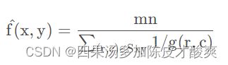
谐波平均滤波器既能处理盐粒噪声(白色噪点)，又能处理类似于高斯噪声的其他噪声，但不能处理胡椒噪声(黑色噪点)。

2.1.4 反谐波平均滤波器

反谐波平均滤波器适用于降低或消除椒盐噪声，计算公式如下：

Q 称为滤波器的阶数，Q 取正整数时可以消除胡椒噪声，Q 取负整数时可以消除盐粒噪声，但不能同时消除这两种噪声。

反谐波平均滤波器当 Q=0 时简化为算术平均滤波器；当 Q=−1时简化为谐波平均滤波器。

2.2 统计排序滤波器

统计排序滤波器是空间滤波器，其响应是基于滤波器邻域中的像素值的顺序，排序结果决定了滤波器的输出。
统计排序包括中值滤波器、最大值滤波器、最小值滤波器、中点滤波器和修正阿尔法均值滤波器。

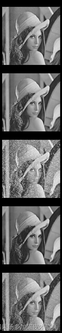
2.2.1 中值滤波器

中值滤波器：用预定义的像素邻域中的灰度中值来代替像素的值，与线性平滑滤波器相比能有效地降低某些随机噪声，且模糊度要小得多。

2.2.2 最大值滤波器

用预定义的像素邻域中的灰度最大值来代替像素的值，可用于找到图像中的最亮点，或用于消弱与明亮区域相邻的暗色区域，也可以用来降低胡椒噪声。

2.2.3 最小值滤波器

最小值滤波器：用预定义的像素邻域中的灰度最小值来代替像素的值，可用于找到图像中的最暗点，或用于削弱与暗色区域相邻的明亮区域，也可以用来降低盐粒噪声。

2.2.4 中点滤波器

中点滤波器：用预定义的像素邻域中的灰度的最大值与最小值的均值来代替像素的值，注意中点的取值与中值常常是不同的。中点滤波器是统计排序滤波器与平均滤波器的结合，适合处理随机分布的噪声，例如高斯噪声、均匀噪声。

"""
统计排序滤波器
"""
import cv2
import matplotlib.pyplot as plt
import numpy as np

img = cv2.imread("./src_data/lenaNoise.png", 0)

img_h = img.shape[0]
img_w = img.shape[1]

m, n = 3, 3
kernalMean = np.ones((m, n), np.float32)  # 生成盒式核

# 边缘填充
hPad = int((m - 1) / 2)
wPad = int((n - 1) / 2)
imgPad = np.pad(img.copy(), ((hPad, m - hPad - 1), (wPad, n - wPad - 1)), mode="edge")

imgMedianFilter = np.zeros(img.shape)  # 中值滤波器
imgMaxFilter = np.zeros(img.shape)  # 最大值滤波器
imgMinFilter = np.zeros(img.shape)  # 最小值滤波器
imgMiddleFilter = np.zeros(img.shape)  # 中点滤波器
for i in range(img_h):
    for j in range(img_w):
        # # 1. 中值滤波器 (median filter)
        pad = imgPad[i:i + m, j:j + n]
        imgMedianFilter[i, j] = np.median(pad)

        # # 2. 最大值滤波器 (maximum filter)
        pad = imgPad[i:i + m, j:j + n]
        imgMaxFilter[i, j] = np.max(pad)

        # # 3. 最小值滤波器 (minimum filter)
        pad = imgPad[i:i + m, j:j + n]
        imgMinFilter[i, j] = np.min(pad)

        # # 4. 中点滤波器 (middle filter)
        pad = imgPad[i:i + m, j:j + n]
        imgMiddleFilter[i, j] = int(pad.max() / 2 + pad.min() / 2)

plt.figure(figsize=(3, 15))
plt.subplot(511), plt.axis('off'), plt.title("origin")
plt.imshow(img, cmap='gray', vmin=0, vmax=255)
plt.subplot(512), plt.axis('off'), plt.title("median filter")
plt.imshow(imgMedianFilter, cmap='gray', vmin=0, vmax=255)
plt.subplot(513), plt.axis('off'), plt.title("maximum filter")
plt.imshow(imgMaxFilter, cmap='gray', vmin=0, vmax=255)
plt.subplot(514), plt.axis('off'), plt.title("minimum filter")
plt.imshow(imgMinFilter, cmap='gray', vmin=0, vmax=255)
plt.subplot(515), plt.axis('off'), plt.title("middle filter")
plt.imshow(imgMiddleFilter, cmap='gray', vmin=0, vmax=255)
plt.tight_layout()
plt.show()

2.2.5 修正阿尔法均值滤波器

修正阿尔法均值滤波器也属于统计排序滤波器，其思想类似于比赛中去掉最高分和最低分后计算平均分。
其计算公式为：

d表示d个最低灰度值和d个最高灰度值，d 的取值范围是[0,mn/2−1]。选择d的大小对图像处理的效果影响很大，当 d=0 时简化为算术平均滤波器，当 d=mn/2−1 简化为中值滤波器。

"""
修正阿尔法均值滤波器
"""
import cv2
import matplotlib.pyplot as plt
import numpy as np

img = cv2.imread("./src_data/lenaNoise.png", 0)

img_h = img.shape[0]
img_w = img.shape[1]

m, n = 5, 5
kernalMean = np.ones((m, n), np.float32)  # 生成盒式核

# 边缘填充
hPad = int((m - 1) / 2)
wPad = int((n - 1) / 2)
imgPad = np.pad(img.copy(), ((hPad, m - hPad - 1), (wPad, n - wPad - 1)), mode="edge")

imgAlphaFilter0 = np.zeros(img.shape)
imgAlphaFilter1 = np.zeros(img.shape)
imgAlphaFilter2 = np.zeros(img.shape)
for i in range(img_h):
    for j in range(img_w):
        # 邻域 m * n
        pad = imgPad[i:i + m, j:j + n]
        padSort = np.sort(pad.flatten())  # 对邻域像素按灰度值排序

        d = 1
        sumAlpha = np.sum(padSort[d:m * n - d - 1])  # 删除 d 个最大灰度值, d 个最小灰度值
        imgAlphaFilter0[i, j] = sumAlpha / (m * n - 2 * d)  # 对剩余像素进行算术平均

        d = 2
        sumAlpha = np.sum(padSort[d:m * n - d - 1])
        imgAlphaFilter1[i, j] = sumAlpha / (m * n - 2 * d)

        d = 4
        sumAlpha = np.sum(padSort[d:m * n - d - 1])
        imgAlphaFilter2[i, j] = sumAlpha / (m * n - 2 * d)

plt.figure(figsize=(9, 7))
plt.subplot(221), plt.axis('off'), plt.title("Original")
plt.imshow(img, cmap='gray', vmin=0, vmax=255)
plt.subplot(222), plt.axis('off'), plt.title("Modified alpha-mean(d=1)")
plt.imshow(imgAlphaFilter0, cmap='gray', vmin=0, vmax=255)
plt.subplot(223), plt.axis('off'), plt.title("Modified alpha-mean(d=2)")
plt.imshow(imgAlphaFilter1, cmap='gray', vmin=0, vmax=255)
plt.subplot(224), plt.axis('off'), plt.title("Modified alpha-mean(d=4)")
plt.imshow(imgAlphaFilter2, cmap='gray', vmin=0, vmax=255)
plt.tight_layout()
plt.show()

2.3 自适应滤波器

前述滤波器直接应用到图像处理，并未考虑图像本身的特征。自适应滤波器的特性根据$m\ast n$矩形邻域$S_{xy}$定义的滤波区域内的图像的统计特性变化。通常，自适应滤波器的性能优于前述的滤波器，但滤波器的复杂度和计算量也更大。
均值和方差是随机变量最基础的统计量。在图像处理中，均值是像素邻域的平均灰度，方差是像素邻域的图像对比度。
令$S_{xy}$表示中心在点$(x,y)$、大小为$(m\ast n)$的矩形子窗口（邻域）,滤波器在由$S_{xy}$定义的邻域操作。
噪声图像在点 $(x,y)$ 的值$g(x,y)$，噪声的方差 ${\sigma }_{\eta }^2$由噪声图像估计；$S_{xy}$中像素的局部平均灰度为 ${\bar{z}}_{S_{xy}}$ ，灰度的局部方差为 ${\sigma }_{S_{xy}}^2$。使用自适应局部降噪滤波器复原的图像 $\hat{f}$在点 $(x,y)$的值，由如下自适应表达式描述：
$$\hat{f}(x,y)=g(x,y)-\frac{{\sigma }_{\eta }^2}{{\sigma }_{S_{xy}}^2}[g(x,y)-{\bar{z}}_{S_{xy}}]$$

自适应局部滤波示例：

# 9.14: 自适应局部降噪滤波器 (Adaptive local noise reduction filter)
img = cv2.imread("./DIP4E/circuitboard-pepper.tif", 0)  # flags=0 读取为灰度图像
hImg = img.shape[0]
wImg = img.shape[1]

m, n = 5, 5
imgAriMean = cv2.boxFilter(img, -1, (m, n))  # 算术平均滤波

# 边缘填充
hPad = int((m-1) / 2)
wPad = int((n-1) / 2)
imgPad = np.pad(img.copy(), ((hPad, m-hPad-1), (wPad, n-wPad-1)), mode="edge")

# 估计原始图像的噪声方差 sigmaEta
mean, stddev = cv2.meanStdDev(img)
sigmaEta = stddev ** 2
print(sigmaEta)

# 自适应局部降噪
epsilon = 1e-8
imgAdaLocal = np.zeros(img.shape)
for i in range(hImg):
    for j in range(wImg):
        pad = imgPad[i:i+m, j:j+n]  # 邻域 Sxy, m*n
        gxy = img[i,j]  # 含噪声图像的像素点
        zSxy = np.mean(pad)  # 局部平均灰度
        sigmaSxy = np.var(pad)  # 灰度的局部方差
        rateSigma = min(sigmaEta / (sigmaSxy + epsilon), 1.0)  # 加性噪声假设：sigmaEta/sigmaSxy < 1
        imgAdaLocal[i, j] = gxy - rateSigma * (gxy - zSxy)

plt.figure(figsize=(9, 6))
plt.subplot(131), plt.axis('off'), plt.title("Original")
plt.imshow(img, cmap='gray', vmin=0, vmax=255)
plt.subplot(132), plt.axis('off'), plt.title("Arithmentic mean filter")
plt.imshow(imgAriMean, cmap='gray', vmin=0, vmax=255)
plt.subplot(133), plt.axis('off'), plt.title("Adaptive local filter")
plt.imshow(imgAdaLocal, cmap='gray', vmin=0, vmax=255)
plt.tight_layout()
plt.show()