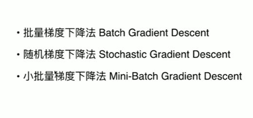
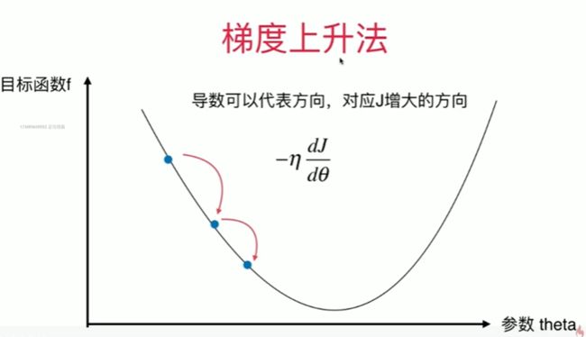
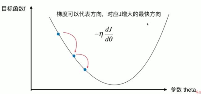
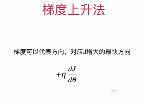
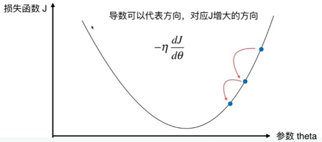
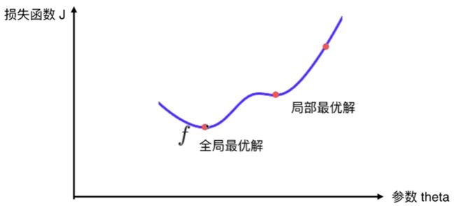
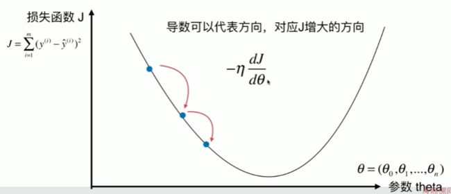
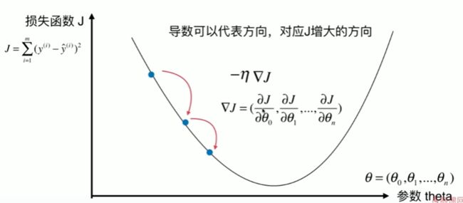
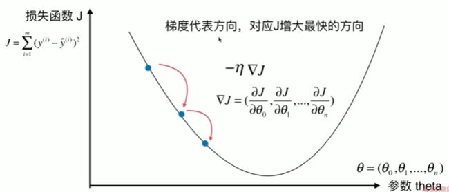
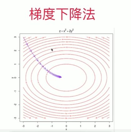
6-1 什么是梯度下降法

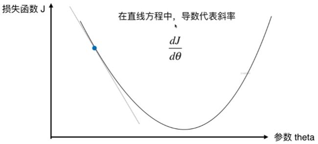
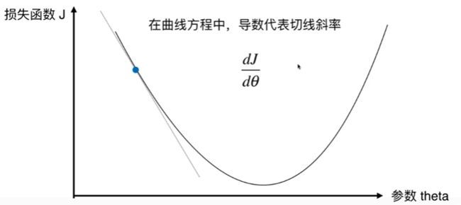
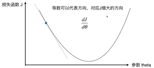
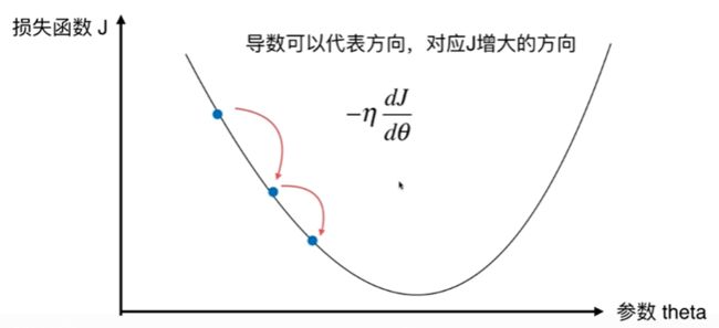


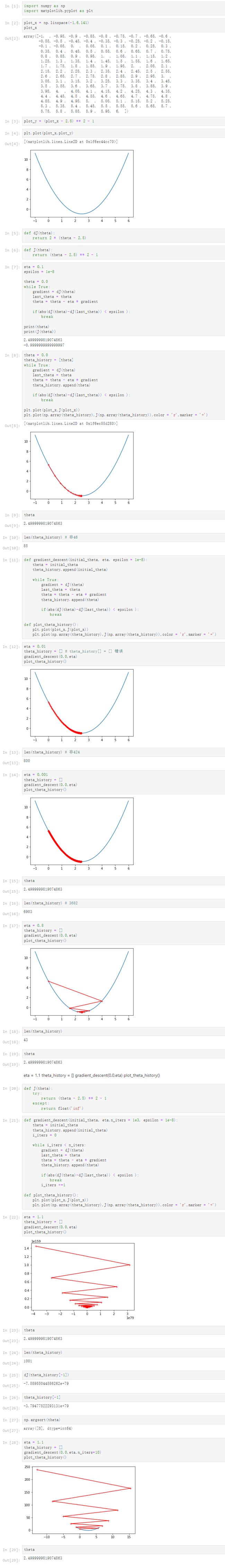
6-2 模拟实现梯度下降法
Notbook 示例
Notbook 源码
[1]
import numpy as np
import matplotlib.pyplot as plt
[2]
plot_x = np.linspace(-1,6,141)
plot_x
array([-1.  , -0.95, -0.9 , -0.85, -0.8 , -0.75, -0.7 , -0.65, -0.6 ,
       -0.55, -0.5 , -0.45, -0.4 , -0.35, -0.3 , -0.25, -0.2 , -0.15,
       -0.1 , -0.05,  0.  ,  0.05,  0.1 ,  0.15,  0.2 ,  0.25,  0.3 ,
        0.35,  0.4 ,  0.45,  0.5 ,  0.55,  0.6 ,  0.65,  0.7 ,  0.75,
        0.8 ,  0.85,  0.9 ,  0.95,  1.  ,  1.05,  1.1 ,  1.15,  1.2 ,
        1.25,  1.3 ,  1.35,  1.4 ,  1.45,  1.5 ,  1.55,  1.6 ,  1.65,
        1.7 ,  1.75,  1.8 ,  1.85,  1.9 ,  1.95,  2.  ,  2.05,  2.1 ,
        2.15,  2.2 ,  2.25,  2.3 ,  2.35,  2.4 ,  2.45,  2.5 ,  2.55,
        2.6 ,  2.65,  2.7 ,  2.75,  2.8 ,  2.85,  2.9 ,  2.95,  3.  ,
        3.05,  3.1 ,  3.15,  3.2 ,  3.25,  3.3 ,  3.35,  3.4 ,  3.45,
        3.5 ,  3.55,  3.6 ,  3.65,  3.7 ,  3.75,  3.8 ,  3.85,  3.9 ,
        3.95,  4.  ,  4.05,  4.1 ,  4.15,  4.2 ,  4.25,  4.3 ,  4.35,
        4.4 ,  4.45,  4.5 ,  4.55,  4.6 ,  4.65,  4.7 ,  4.75,  4.8 ,
        4.85,  4.9 ,  4.95,  5.  ,  5.05,  5.1 ,  5.15,  5.2 ,  5.25,
        5.3 ,  5.35,  5.4 ,  5.45,  5.5 ,  5.55,  5.6 ,  5.65,  5.7 ,
        5.75,  5.8 ,  5.85,  5.9 ,  5.95,  6.  ])
[3]
plot_y = (plot_x - 2.5) ** 2 - 1
[4]
plt.plot(plot_x,plot_y)
[]

[5]
def dJ(theta):
    return 2 * (theta - 2.5)
[6]
def J(theta):
    return (theta - 2.5) ** 2 - 1
[7]
eta = 0.1
epsilon = 1e-8

theta = 0.0
while True:
    gradient = dJ(theta)
    last_theta = theta
    theta = theta - eta * gradient

    if(abs(dJ(theta)-dJ(last_theta)) < epsilon ):
        break

print(theta)
print(J(theta))
2.4999999819074863
-0.9999999999999997

[8]
theta = 0.0
theta_history = [theta]
while True:
    gradient = dJ(theta)
    last_theta = theta
    theta = theta - eta * gradient
    theta_history.append(theta)

    if(abs(dJ(theta)-dJ(last_theta)) < epsilon ):
        break

plt.plot(plot_x,J(plot_x))
plt.plot(np.array(theta_history),J(np.array(theta_history)),color = 'r',marker = '+')
[]

[9]
theta
2.4999999819074863
[10]
len(theta_history) # 非46
85
[11]
def gradient_descent(initial_theta, eta, epsilon = 1e-8):
    theta = initial_theta
    theta_history.append(initial_theta)

    while True:
        gradient = dJ(theta)
        last_theta = theta
        theta = theta - eta * gradient
        theta_history.append(theta)

        if(abs(dJ(theta)-dJ(last_theta)) < epsilon ):
            break

def plot_theta_history():
    plt.plot(plot_x,J(plot_x))
    plt.plot(np.array(theta_history),J(np.array(theta_history)),color = 'r',marker = '+')
[12]
eta = 0.01
theta_history = [] # theta_history[] = [] 错误
gradient_descent(0.0,eta)
plot_theta_history()

[13]
len(theta_history) # 非424
800
[14]
eta = 0.001
theta_history = []
gradient_descent(0.0,eta)
plot_theta_history()

[15]
theta
2.4999999819074863
[16]
len(theta_history) # 3682
6903
[17]
eta = 0.8
theta_history = []
gradient_descent(0.0,eta)
plot_theta_history()

[18]
len(theta_history)
43
[19]
theta
2.4999999819074863
eta = 1.1 theta_history = [] gradient_descent(0.0,eta) plot_theta_history()

[20]
def J(theta):
    try:
        return (theta - 2.5) ** 2 - 1
    except:
        return float('inf')
[21]
def gradient_descent(initial_theta, eta,n_iters = 1e3, epsilon = 1e-8):
    theta = initial_theta
    theta_history.append(initial_theta)
    i_iters = 0

    while i_iters < n_iters:
        gradient = dJ(theta)
        last_theta = theta
        theta = theta - eta * gradient
        theta_history.append(theta)

        if(abs(dJ(theta)-dJ(last_theta)) < epsilon ):
            break
        i_iters +=1

def plot_theta_history():
    plt.plot(plot_x,J(plot_x))
    plt.plot(np.array(theta_history),J(np.array(theta_history)),color = 'r',marker = '+')
[22]
eta = 1.1
theta_history = []
gradient_descent(0.0,eta)
plot_theta_history()

[23]
theta
2.4999999819074863
[24]
len(theta_history)
1001
[25]
dJ(theta_history[-1])
-7.58955044586262e+79
[26]
theta_history[-1]
-3.79477522293131e+79
[27]
np.argsort(theta)
array([0], dtype=int64)
[28]
eta = 1.1
theta_history = []
gradient_descent(0.0,eta,n_iters=10)
plot_theta_history()

[29]
theta
2.4999999819074863
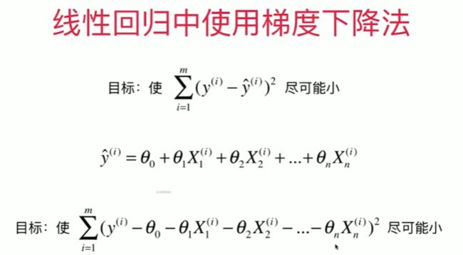
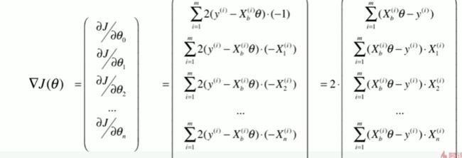
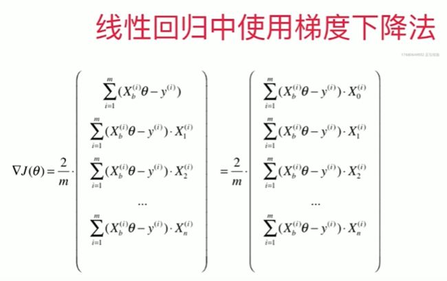
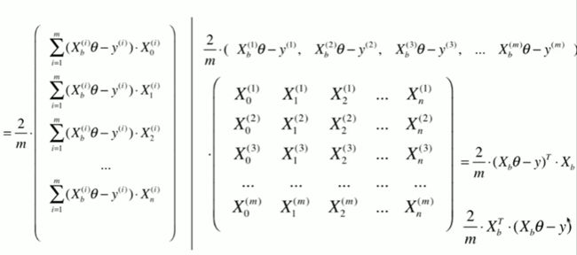
6-3 线性回归中的梯度下降法
6-4 实现线性回归中的梯度下降法
Notbook 示例
Notbook 源码
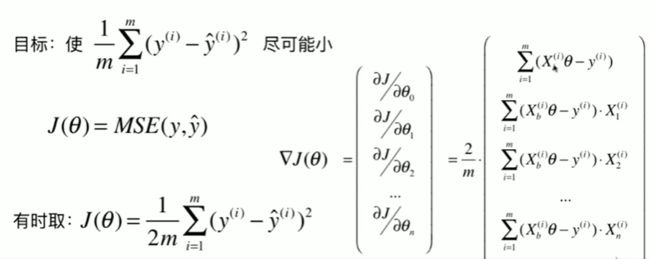
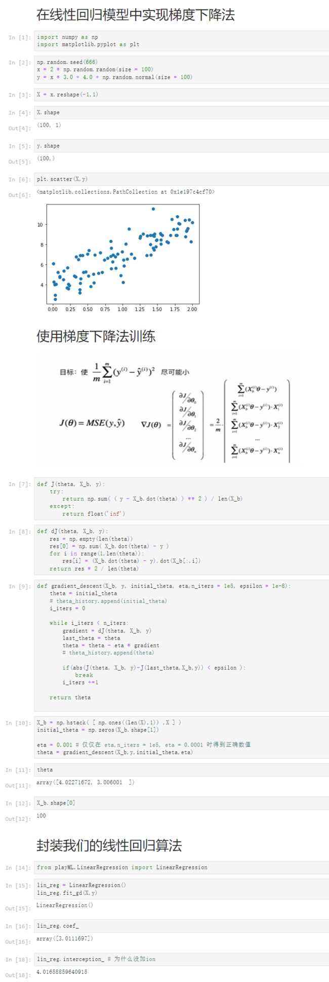
在线性回归模型中实现梯度下降法
[1]
import numpy as np
import matplotlib.pyplot as plt
[2]
np.random.seed(666)
x = 2 * np.random.random(size = 100)
y = x * 3.0 + 4.0 + np.random.normal(size = 100)
[3]
X = x.reshape(-1,1)
[4]
X.shape
(100, 1)
[5]
y.shape
(100,)
[6]
plt.scatter(X,y)


使用梯度下降法训练
%E6%A2%AF%E5%BA%A6%E4%B8%8B%E9%99%8D.png

[7]
def J(theta, X_b, y):
    try:
        return np.sum( ( y - X_b.dot(theta) ) ** 2 ) / len(X_b)
    except:
        return float('inf')
[8]
def dJ(theta, X_b, y):
    res = np.empty(len(theta))
    res[0] = np.sum( X_b.dot(theta) - y )
    for i in range(1,len(theta)):
        res[i] = (X_b.dot(theta) - y).dot(X_b[:,i])
    return res * 2 / len(theta)
[9]
def gradient_descent(X_b, y, initial_theta, eta,n_iters = 1e5, epsilon = 1e-8):
    theta = initial_theta
    # theta_history.append(initial_theta)
    i_iters = 0

    while i_iters < n_iters:
        gradient = dJ(theta, X_b, y)
        last_theta = theta
        theta = theta - eta * gradient
        # theta_history.append(theta)

        if(abs(J(theta, X_b, y)-J(last_theta,X_b,y)) < epsilon ):
            break
        i_iters +=1

    return theta

[10]
X_b = np.hstack( [ np.ones((len(X),1)) ,X ] )
initial_theta = np.zeros(X_b.shape[1])

eta = 0.001 # 仅仅在 eta,n_iters = 1e5, eta = 0.0001 时得到正确数值
theta = gradient_descent(X_b,y,initial_theta,eta)
[11]
theta
array([4.02271672, 3.006001  ])
[12]
X_b.shape[0]
100
封装我们的线性回归算法
[14]
from playML.LinearRegression import LinearRegression
[15]
lin_reg = LinearRegression()
lin_reg.fit_gd(X,y)
LinearRegression()
[16]
lin_reg.coef_
array([3.0111697])
[18]
lin_reg.interception_ # 为什么没加ion
4.01658859640915
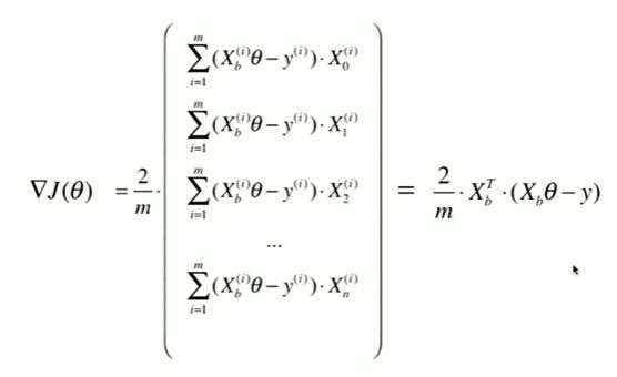
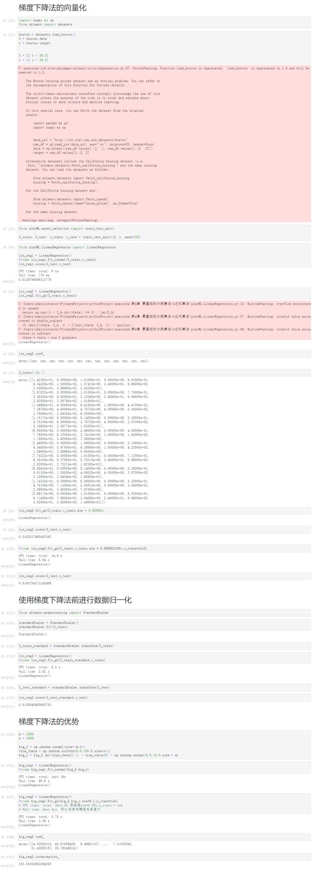
6-5 梯度下降的向量化和数据标准化

Notbook 示例
Notbook 源码
梯度下降法的向量化
[1]
import numpy as np
from sklearn import datasets
[2]
boston = datasets.load_boston()
X = boston.data
y = boston.target


X = X[ y < 50.0]
y = y[ y < 50.0]
F:\anaconda\lib\site-packages\sklearn\utils\deprecation.py:87: FutureWarning: Function load_boston is deprecated; `load_boston` is deprecated in 1.0 and will be removed in 1.2.

    The Boston housing prices dataset has an ethical problem. You can refer to
    the documentation of this function for further details.

    The scikit-learn maintainers therefore strongly discourage the use of this
    dataset unless the purpose of the code is to study and educate about
    ethical issues in data science and machine learning.

    In this special case, you can fetch the dataset from the original
    source::

        import pandas as pd
        import numpy as np


        data_url = "http://lib.stat.cmu.edu/datasets/boston"
        raw_df = pd.read_csv(data_url, sep="\s+", skiprows=22, header=None)
        data = np.hstack([raw_df.values[::2, :], raw_df.values[1::2, :2]])
        target = raw_df.values[1::2, 2]

    Alternative datasets include the California housing dataset (i.e.
    :func:`~sklearn.datasets.fetch_california_housing`) and the Ames housing
    dataset. You can load the datasets as follows::

        from sklearn.datasets import fetch_california_housing
        housing = fetch_california_housing()

    for the California housing dataset and::

        from sklearn.datasets import fetch_openml
        housing = fetch_openml(name="house_prices", as_frame=True)

    for the Ames housing dataset.

  warnings.warn(msg, category=FutureWarning)

[3]
from playML.model_selection import train_test_split

X_train, X_test, y_train, y_test = train_test_split(X, y, seed=222)
[4]
from playML.LinearRegression import LinearRegression

lin_reg1 = LinearRegression()
%time lin_reg1.fit_normal(X_train,y_train)
lin_reg1.score(X_test,y_test)
CPU times: total: 0 ns
Wall time: 770 ms

0.8129794056212779
[5]
lin_reg2 = LinearRegression()
lin_reg2.fit_gd(X_train,y_train)
C:\Users\Administrator\PycharmProjects\pythonProject\anaconda\第4章 最基础的分类算法-k近邻算法\playML\LinearRegression.py:33: RuntimeWarning: overflow encountered in square
  return np.sum((y - X_b.dot(theta)) ** 2) / len(X_b)
C:\Users\Administrator\PycharmProjects\pythonProject\anaconda\第4章 最基础的分类算法-k近邻算法\playML\LinearRegression.py:57: RuntimeWarning: invalid value encountered in double_scalars
  if (abs(J(theta, X_b, y) - J(last_theta, X_b, y)) < epsilon):
C:\Users\Administrator\PycharmProjects\pythonProject\anaconda\第4章 最基础的分类算法-k近邻算法\playML\LinearRegression.py:54: RuntimeWarning: invalid value encountered in subtract
  theta = theta - eta * gradient

LinearRegression()
[6]
lin_reg2.coef_
array([nan, nan, nan, nan, nan, nan, nan, nan, nan, nan, nan, nan, nan])
[7]
X_train[:10,:]
array([[1.42362e+01, 0.00000e+00, 1.81000e+01, 0.00000e+00, 6.93000e-01,
        6.34300e+00, 1.00000e+02, 1.57410e+00, 2.40000e+01, 6.66000e+02,
        2.02000e+01, 3.96900e+02, 2.03200e+01],
       [3.67822e+00, 0.00000e+00, 1.81000e+01, 0.00000e+00, 7.70000e-01,
        5.36200e+00, 9.62000e+01, 2.10360e+00, 2.40000e+01, 6.66000e+02,
        2.02000e+01, 3.80790e+02, 1.01900e+01],
       [1.04690e-01, 4.00000e+01, 6.41000e+00, 1.00000e+00, 4.47000e-01,
        7.26700e+00, 4.90000e+01, 4.78720e+00, 4.00000e+00, 2.54000e+02,
        1.76000e+01, 3.89250e+02, 6.05000e+00],
       [1.15172e+00, 0.00000e+00, 8.14000e+00, 0.00000e+00, 5.38000e-01,
        5.70100e+00, 9.50000e+01, 3.78720e+00, 4.00000e+00, 3.07000e+02,
        2.10000e+01, 3.58770e+02, 1.83500e+01],
       [6.58800e-02, 0.00000e+00, 2.46000e+00, 0.00000e+00, 4.88000e-01,
        7.76500e+00, 8.33000e+01, 2.74100e+00, 3.00000e+00, 1.93000e+02,
        1.78000e+01, 3.95560e+02, 7.56000e+00],
       [2.49800e-02, 0.00000e+00, 1.89000e+00, 0.00000e+00, 5.18000e-01,
        6.54000e+00, 5.97000e+01, 6.26690e+00, 1.00000e+00, 4.22000e+02,
        1.59000e+01, 3.89960e+02, 8.65000e+00],
       [7.75223e+00, 0.00000e+00, 1.81000e+01, 0.00000e+00, 7.13000e-01,
        6.30100e+00, 8.37000e+01, 2.78310e+00, 2.40000e+01, 6.66000e+02,
        2.02000e+01, 2.72210e+02, 1.62300e+01],
       [9.88430e-01, 0.00000e+00, 8.14000e+00, 0.00000e+00, 5.38000e-01,
        5.81300e+00, 1.00000e+02, 4.09520e+00, 4.00000e+00, 3.07000e+02,
        2.10000e+01, 3.94540e+02, 1.98800e+01],
       [1.14320e-01, 0.00000e+00, 8.56000e+00, 0.00000e+00, 5.20000e-01,
        6.78100e+00, 7.13000e+01, 2.85610e+00, 5.00000e+00, 3.84000e+02,
        2.09000e+01, 3.95580e+02, 7.67000e+00],
       [5.69175e+00, 0.00000e+00, 1.81000e+01, 0.00000e+00, 5.83000e-01,
        6.11400e+00, 7.98000e+01, 3.54590e+00, 2.40000e+01, 6.66000e+02,
        2.02000e+01, 3.92680e+02, 1.49800e+01]])
[8]
lin_reg2.fit_gd(X_train,y_train,eta = 0.000001)
LinearRegression()
[9]
lin_reg2.score(X_test,y_test)
0.5183037995455362
[10]
%time lin_reg2.fit_gd(X_train,y_train,eta = 0.0000031001,n_iters=1e12)
CPU times: total: 14.9 s
Wall time: 8.04 s

LinearRegression()
[11]
lin_reg2.score(X_test,y_test)
0.6180704373142486
使用梯度下降法前进行数据归一化
[12]
from sklearn.preprocessing import StandardScaler
[13]
standardScaler = StandardScaler()
standardScaler.fit(X_train)
StandardScaler()
[14]
X_train_standard = standardScaler.transform(X_train)
[15]
lin_reg3 = LinearRegression()
%time lin_reg3.fit_gd(X_train_standard,y_train)
CPU times: total: 5.5 s
Wall time: 2.82 s

LinearRegression()
[16]
X_test_standard = standardScaler.transform(X_test)
[17]
lin_reg3.score(X_test_standard,y_test)
0.8130040900692703
梯度下降法的优势
[18]
m = 2000
n = 5000

big_X = np.random.normal(size=(m,n))
true_theta = np.random.uniform(0.0,100.0,size=n+1)
big_y = big_X.dot(true_theta[1:]) + true_theta[0] + np.random.normal(0.0,10.0,size = m)
[19]
big_reg1 = LinearRegression()
%time big_reg1.fit_normal(big_X,big_y)
CPU times: total: 1min 19s
Wall time: 46.6 s

LinearRegression()
[29]
big_reg2 = LinearRegression()
%time big_reg2.fit_gd(big_X,big_y,eta=0.1,n_iters=1e3)
# CPU times: total: 8min 8s 原因是eta=0.001,n_iters = 1e4
# Wall time: 5min 41s  所以与具体模型关系甚大
CPU times: total: 5.75 s
Wall time: 3.29 s

LinearRegression()
[30]
big_reg2.coef_
array([14.82820315, 43.97009426,  6.49921157, ...,  7.31030043,
       51.42885153, 20.76248914])
[31]
big_reg2.interception_
102.55282983264055
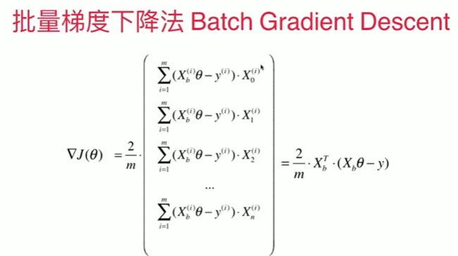
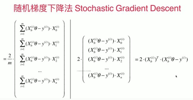
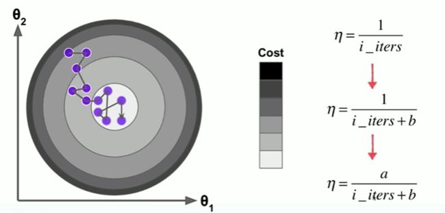
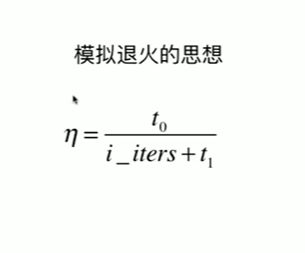
6-6 随机梯度下降法
Notbook 示例
Notbook 源码
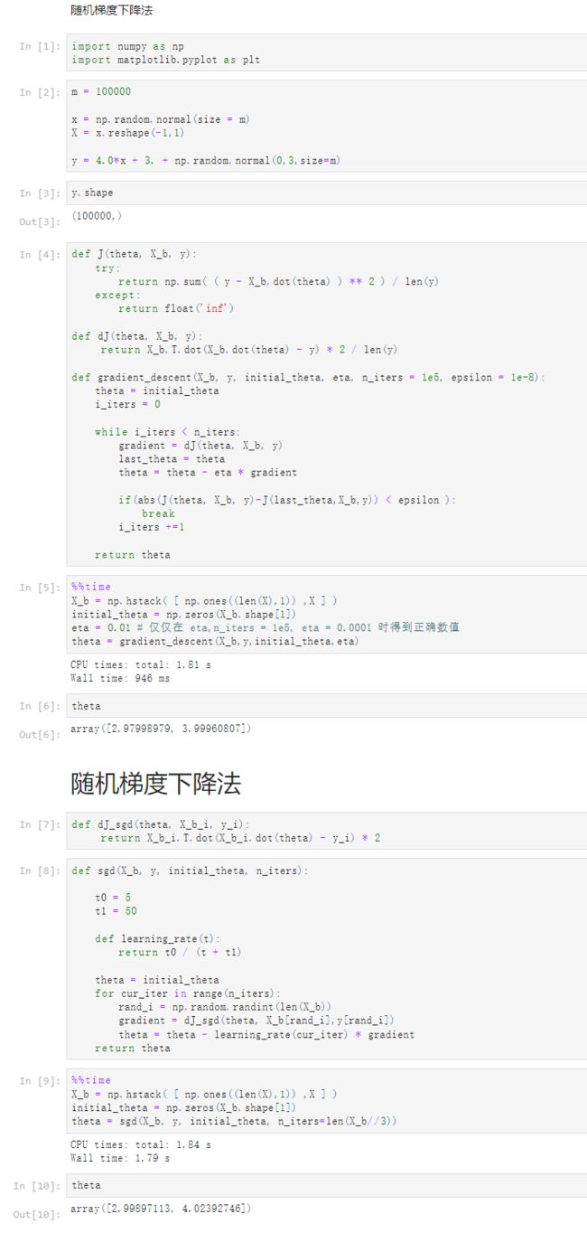
随机梯度下降法

[1]
import numpy as np
import matplotlib.pyplot as plt
[2]
m = 100000

x = np.random.normal(size = m)
X = x.reshape(-1,1)

y = 4.0*x + 3. + np.random.normal(0,3,size=m)
[3]
y.shape
(100000,)
[4]
def J(theta, X_b, y):
    try:
        return np.sum( ( y - X_b.dot(theta) ) ** 2 ) / len(y)
    except:
        return float('inf')

def dJ(theta, X_b, y):
     return X_b.T.dot(X_b.dot(theta) - y) * 2 / len(y)

def gradient_descent(X_b, y, initial_theta, eta, n_iters = 1e5, epsilon = 1e-8):
    theta = initial_theta
    i_iters = 0

    while i_iters < n_iters:
        gradient = dJ(theta, X_b, y)
        last_theta = theta
        theta = theta - eta * gradient

        if(abs(J(theta, X_b, y)-J(last_theta,X_b,y)) < epsilon ):
            break
        i_iters +=1

    return theta
[5]
%%time
X_b = np.hstack( [ np.ones((len(X),1)) ,X ] )
initial_theta = np.zeros(X_b.shape[1])
eta = 0.01 # 仅仅在 eta,n_iters = 1e5, eta = 0.0001 时得到正确数值
theta = gradient_descent(X_b,y,initial_theta,eta)
CPU times: total: 1.81 s
Wall time: 946 ms

[6]
theta
array([2.97998979, 3.99960807])
随机梯度下降法
[7]
def dJ_sgd(theta, X_b_i, y_i):
     return X_b_i.T.dot(X_b_i.dot(theta) - y_i) * 2
[8]
def sgd(X_b, y, initial_theta, n_iters):

    t0 = 5
    t1 = 50

    def learning_rate(t):
        return t0 / (t + t1)

    theta = initial_theta
    for cur_iter in range(n_iters):
        rand_i = np.random.randint(len(X_b))
        gradient = dJ_sgd(theta, X_b[rand_i],y[rand_i])
        theta = theta - learning_rate(cur_iter) * gradient
    return theta
[9]
%%time
X_b = np.hstack( [ np.ones((len(X),1)) ,X ] )
initial_theta = np.zeros(X_b.shape[1])
theta = sgd(X_b, y, initial_theta, n_iters=len(X_b//3))
CPU times: total: 1.84 s
Wall time: 1.79 s

[10]
theta
array([2.99897113, 4.02392746])
6-7 scikit-learn中的随机梯度下降法
Notbook 示例
Notbook 源码
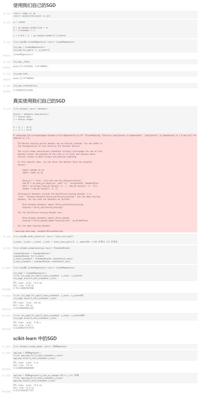
使用我们自己的SGD
[1]
import numpy as np
import matplotlib.pyplot as plt
[2]
m = 100000

x = np.random.normal(size = m)
X = x.reshape(-1,1)

y = 4.0*x + 3. + np.random.normal(0,3,size=m)
[3]
from playML.LinearRegression import LinearRegression

lin_reg = LinearRegression()
lin_reg.fit_sgd(X, y, n_iters=2)
LinearRegression()
[4]
lin_reg._theta
array([3.01202028, 3.97799884])
[5]
lin_reg.coef_
array([3.97799884])
[6]
lin_reg.interception_
3.012020275313304
真实使用我们自己的SGD
[7]
from sklearn import datasets

boston = datasets.load_boston()
X = boston.data
y = boston.target


X = X[ y < 50.0]
y = y[ y < 50.0]
F:\anaconda\lib\site-packages\sklearn\utils\deprecation.py:87: FutureWarning: Function load_boston is deprecated; `load_boston` is deprecated in 1.0 and will be removed in 1.2.

    The Boston housing prices dataset has an ethical problem. You can refer to
    the documentation of this function for further details.

    The scikit-learn maintainers therefore strongly discourage the use of this
    dataset unless the purpose of the code is to study and educate about
    ethical issues in data science and machine learning.

    In this special case, you can fetch the dataset from the original
    source::

        import pandas as pd
        import numpy as np


        data_url = "http://lib.stat.cmu.edu/datasets/boston"
        raw_df = pd.read_csv(data_url, sep="\s+", skiprows=22, header=None)
        data = np.hstack([raw_df.values[::2, :], raw_df.values[1::2, :2]])
        target = raw_df.values[1::2, 2]

    Alternative datasets include the California housing dataset (i.e.
    :func:`~sklearn.datasets.fetch_california_housing`) and the Ames housing
    dataset. You can load the datasets as follows::

        from sklearn.datasets import fetch_california_housing
        housing = fetch_california_housing()

    for the California housing dataset and::

        from sklearn.datasets import fetch_openml
        housing = fetch_openml(name="house_prices", as_frame=True)

    for the Ames housing dataset.

  warnings.warn(msg, category=FutureWarning)

[8]
from playML.model_selection import train_test_split

X_train, X_test, y_train, y_test = train_test_split(X, y, seed=666) # 666 效果比 222 好很多
[9]
from sklearn.preprocessing import StandardScaler

standardScaler = StandardScaler()
standardScaler.fit(X_train)
X_train_standard = standardScaler.transform(X_train)
X_test_standard = standardScaler.transform(X_test)
[10]
from playML.LinearRegression import LinearRegression

lin_reg2 = LinearRegression()
%time lin_reg2.fit_sgd(X_train_standard, y_train, n_iters=2)
lin_reg2.score(X_test_standard,y_test)
CPU times: total: 15.6 ms
Wall time: 8.98 ms

0.7911189802097699
[11]
%time lin_reg2.fit_sgd(X_train_standard, y_train, n_iters=50)
lin_reg2.score(X_test_standard,y_test)
CPU times: total: 219 ms
Wall time: 226 ms

0.8132588958621522
[13]
%time lin_reg2.fit_sgd(X_train_standard, y_train, n_iters=500)
lin_reg2.score(X_test_standard,y_test)
CPU times: total: 2.09 s
Wall time: 2.93 s

0.8129564757875579
scikit-learn 中的SGD
[14]
from sklearn.linear_model import SGDRegressor
[15]
sgd_reg = SGDRegressor()
%time sgd_reg.fit(X_train_standard,y_train)
sgd_reg.score(X_test_standard,y_test)
CPU times: total: 0 ns
Wall time: 116 ms

0.8129895569490898
[18]
sgd_reg = SGDRegressor(n_iter_no_change=100)# n_iter 报错
%time sgd_reg.fit(X_train_standard,y_train)
sgd_reg.score(X_test_standard,y_test)
CPU times: total: 15.6 ms
Wall time: 22.9 ms

0.8131520202077357
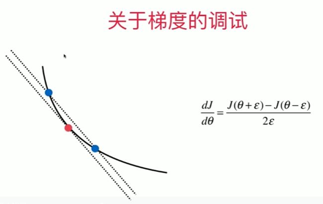
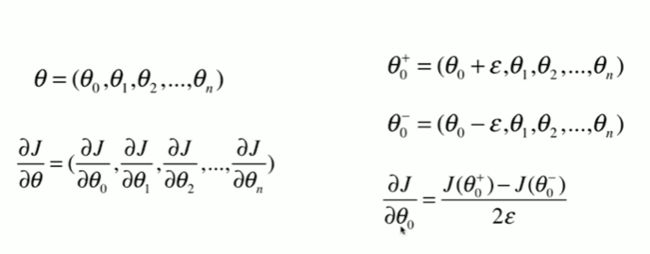
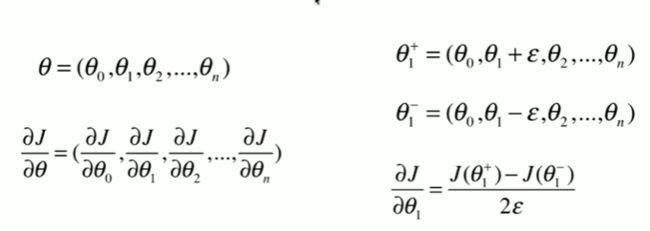
6-8 如何确定梯度计算的准确性 调试梯度下降法
Notbook 示例
Notbook 源码
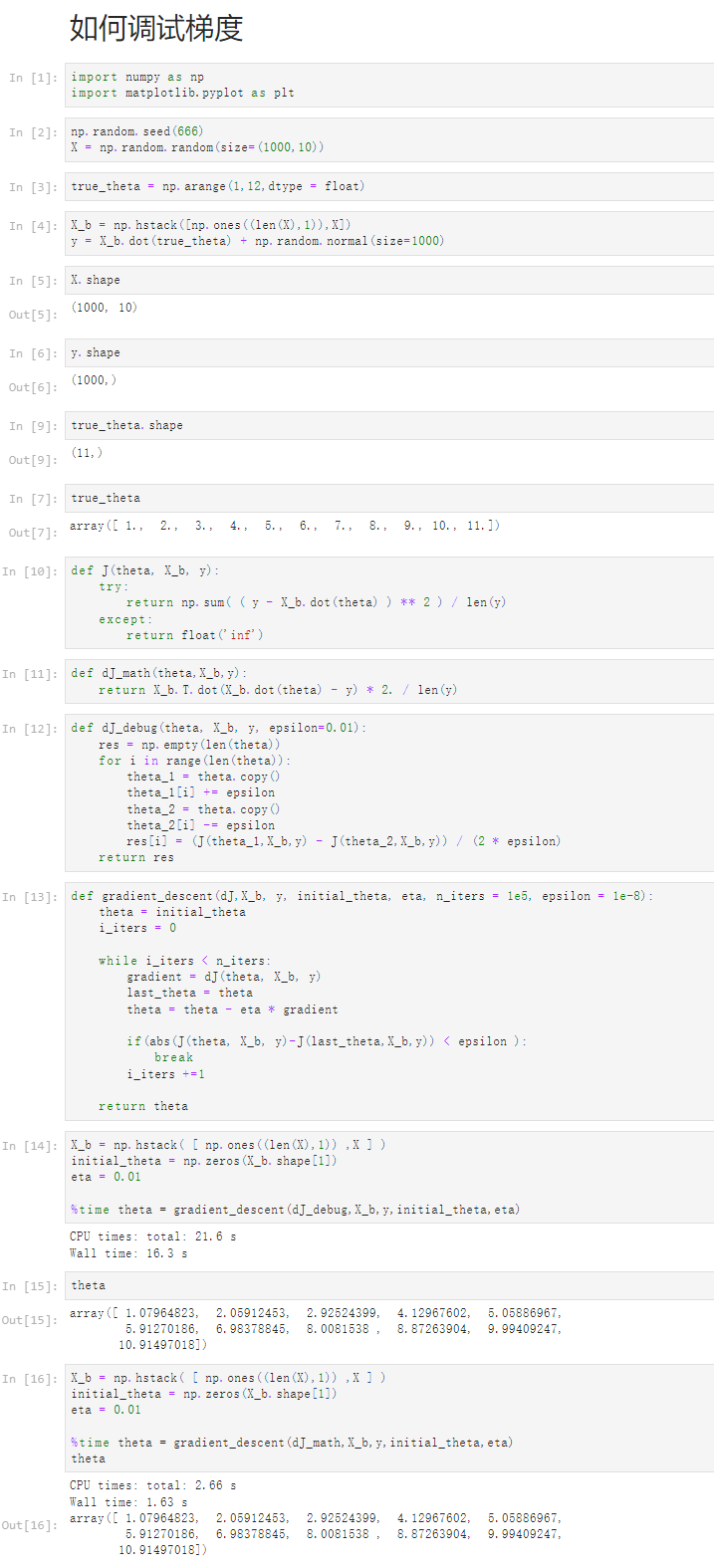
如何调试梯度
[1]
import numpy as np
import matplotlib.pyplot as plt
[2]
np.random.seed(666)
X = np.random.random(size=(1000,10))
[3]
true_theta = np.arange(1,12,dtype = float)
[4]
X_b = np.hstack([np.ones((len(X),1)),X])
y = X_b.dot(true_theta) + np.random.normal(size=1000)
[5]
X.shape
(1000, 10)
[6]
y.shape
(1000,)
[9]
true_theta.shape
(11,)
[7]
true_theta
array([ 1.,  2.,  3.,  4.,  5.,  6.,  7.,  8.,  9., 10., 11.])
[10]
def J(theta, X_b, y):
    try:
        return np.sum( ( y - X_b.dot(theta) ) ** 2 ) / len(y)
    except:
        return float('inf')
[11]
def dJ_math(theta,X_b,y):
    return X_b.T.dot(X_b.dot(theta) - y) * 2. / len(y)
[12]
def dJ_debug(theta, X_b, y, epsilon=0.01):
    res = np.empty(len(theta))
    for i in range(len(theta)):
        theta_1 = theta.copy()
        theta_1[i] += epsilon
        theta_2 = theta.copy()
        theta_2[i] -= epsilon
        res[i] = (J(theta_1,X_b,y) - J(theta_2,X_b,y)) / (2 * epsilon)
    return res
[13]
def gradient_descent(dJ,X_b, y, initial_theta, eta, n_iters = 1e5, epsilon = 1e-8):
    theta = initial_theta
    i_iters = 0

    while i_iters < n_iters:
        gradient = dJ(theta, X_b, y)
        last_theta = theta
        theta = theta - eta * gradient

        if(abs(J(theta, X_b, y)-J(last_theta,X_b,y)) < epsilon ):
            break
        i_iters +=1

    return theta
[14]
X_b = np.hstack( [ np.ones((len(X),1)) ,X ] )
initial_theta = np.zeros(X_b.shape[1])
eta = 0.01

%time theta = gradient_descent(dJ_debug,X_b,y,initial_theta,eta)
CPU times: total: 21.6 s
Wall time: 16.3 s

[15]
theta
array([ 1.07964823,  2.05912453,  2.92524399,  4.12967602,  5.05886967,
        5.91270186,  6.98378845,  8.0081538 ,  8.87263904,  9.99409247,
       10.91497018])
[16]
X_b = np.hstack( [ np.ones((len(X),1)) ,X ] )
initial_theta = np.zeros(X_b.shape[1])
eta = 0.01

%time theta = gradient_descent(dJ_math,X_b,y,initial_theta,eta)
theta
CPU times: total: 2.66 s
Wall time: 1.63 s

array([ 1.07964823,  2.05912453,  2.92524399,  4.12967602,  5.05886967,
        5.91270186,  6.98378845,  8.0081538 ,  8.87263904,  9.99409247,
       10.91497018])
6-9 有关梯度下降法的更多深入讨论