sklearn_SVM:处理样本不平衡问题__菜菜视频学习笔记
SVM:处理样本不平衡问题
-
- 1.通过参数class_weight来处理样本不均衡问题
- 2.混淆矩阵(Confusion Matrix)
-
- 2.1精确度
- 2.2 召回率
- 3.3 特异度
- 3.4 假正率
- 3.ROC曲线及其相关问题
-
- 3.1概率&&阈值(threshold)
- 3.2 置信度参数 decision_function,predict_proba
- 3.3 绘制SVM的ROC曲线
- 3.4 sklearn中ROC与AUC
- 3.5 利用ROC曲线寻找最佳阈值
对于软间隔数据来说,需要松弛系数和松弛系数的参数c来平衡“最大边际”与”被分错样本数量“的平衡
硬间隔:决策边界由两个标签不一致的支持向量来决定和最小化损失函数(最大化决策边际)
软间隔 : 软间隔的支持向量可以分布在任意位置
import numpy as np
import matplotlib.pyplot as plt
from matplotlib.colors import ListedColormap
from sklearn import svm
from sklearn.datasets import make_circles, make_moons, make_blobs,make_classification

n_samples = 100

datasets = [
    make_moons(n_samples=n_samples, noise=0.2, random_state=0),
    make_circles(n_samples=n_samples, noise=0.2, factor=0.5, random_state=1),
    make_blobs(n_samples=n_samples, centers=2, random_state=5),
    make_classification(n_samples=n_samples,n_features = 2,n_informative=2,n_redundant=0, random_state=5)
]

Kernel = ["linear"]

#四个数据集分别是什么样子呢?
for X,Y in datasets:
    plt.figure(figsize=(5,4))
    plt.scatter(X[:,0],X[:,1],c=Y,s=50,cmap="rainbow")

nrows=len(datasets)
ncols=len(Kernel) + 1

fig, axes = plt.subplots(nrows, ncols,figsize=(10,16))

#第一层循环:在不同的数据集中循环
for ds_cnt, (X,Y) in enumerate(datasets):

    #在图像中的第一列,放置原数据的分布
    ax = axes[ds_cnt, 0]
    if ds_cnt == 0:
        ax.set_title("Input data")
    ax.scatter(X[:, 0], X[:, 1], c=Y, zorder=10, cmap=plt.cm.Paired,edgecolors='k')
    ax.set_xticks(())
    ax.set_yticks(())

    #第二层循环:在不同的核函数中循环
    #从图像的第二列开始,一个个填充分类结果
    for est_idx, kernel in enumerate(Kernel):

        #定义子图位置
        ax = axes[ds_cnt, est_idx + 1]

        #建模
        clf = svm.SVC(kernel=kernel, gamma=2).fit(X, Y)
        score = clf.score(X, Y)

        #绘制图像本身分布的散点图
        ax.scatter(X[:, 0], X[:, 1], c=Y
                   ,zorder=10
                   ,cmap=plt.cm.Paired,edgecolors='k')
        #绘制支持向量
        ax.scatter(clf.support_vectors_[:, 0], clf.support_vectors_[:, 1], s=100,
                    facecolors='none', zorder=10, edgecolors='white')

        #绘制决策边界
        x_min, x_max = X[:, 0].min() - .5, X[:, 0].max() + .5
        y_min, y_max = X[:, 1].min() - .5, X[:, 1].max() + .5

        #np.mgrid,合并了我们之前使用的np.linspace和np.meshgrid的用法
        #一次性使用最大值和最小值来生成网格
        #表示为[起始值:结束值:步长]
        #如果步长是复数,则其整数部分就是起始值和结束值之间创建的点的数量,并且结束值被包含在内
        XX, YY = np.mgrid[x_min:x_max:200j, y_min:y_max:200j]
        #np.c_,类似于np.vstack的功能
        Z = clf.decision_function(np.c_[XX.ravel(), YY.ravel()]).reshape(XX.shape)
        #填充等高线不同区域的颜色
        ax.pcolormesh(XX, YY, Z > 0, cmap=plt.cm.Paired)
        #绘制等高线
        ax.contour(XX, YY, Z, colors=['k', 'k', 'k'], linestyles=['--', '-', '--'],
                    levels=[-1, 0, 1])

        #设定坐标轴为不显示
        ax.set_xticks(())
        ax.set_yticks(())

        #将标题放在第一行的顶上
        if ds_cnt == 0:
            ax.set_title(kernel)

        #为每张图添加分类的分数
        ax.text(0.95, 0.06, ('%.2f' % score).lstrip('0')
                , size=15
                , bbox=dict(boxstyle='round', alpha=0.8, facecolor='white')
                	#为分数添加一个白色的格子作为底色
                , transform=ax.transAxes #确定文字所对应的坐标轴,就是ax子图的坐标轴本身
                , horizontalalignment='right' #位于坐标轴的什么方向
               )

plt.tight_layout()
plt.show()

# 决策边界上的支持向量对应的是平衡最优解对应的支持向量
# 所有的支持向量决定决策边界的位置


1.通过参数class_weight来处理样本不均衡问题
导入需要的库和模块
# 解决样本不均衡问题,svm中使用class_weight,sample_weight
# class_weight ,提升少数类权重使得算法意识到样本是不平衡的
# samplee_weight,对样本的加权重,使决策边界的变形非常明显
# 但是SVM中分类判断依据决策边界决定,决策边界又由参数c来决定,所以解决样本不均衡问题由参数c实现
import numpy as np
import matplotlib.pyplot as plt
from sklearn import svm
from sklearn.datasets import make_blobs
创建样本不均衡的数据集
class_1 = 500 #类别1有500个样本,   10:1
class_2 = 50 #类别2只有50个
centers = [[0.0, 0.0], [2.0, 2.0]] #设定两个类别的中心
clusters_std = [1.5, 0.5] #设定两个类别的方差,通常来说,样本量比较大的类别会更加松散
X, y = make_blobs(n_samples=[class_1, class_2],
                  centers=centers,
                  cluster_std=clusters_std,
                  random_state=0, shuffle=False)
#在一个图上画两个簇
X.shape
(550, 2)
#看看数据集长什么样
plt.scatter(X[:, 0], X[:, 1], c=y, cmap="rainbow",s=10)
plt.show()
#其中红色点是少数类,紫色点是多数类

在数据集上分别建模
#不设定class_weight
clf = svm.SVC(kernel='linear', C=1.0)
clf.fit(X, y)
SVC(kernel='linear')In a Jupyter environment, please rerun this cell to show the HTML representation or trust the notebook.
On GitHub, the HTML representation is unable to render, please try loading this page with nbviewer.org.
SVC
SVC(kernel='linear')
class_weight“平衡”模式使用 y 的值自动调整与输入数据中的类频率成反比的权重,使得少数类获得更大的权重
#设定class_weight
wclf = svm.SVC(kernel='linear', class_weight={1: 10})
wclf.fit(X, y)
SVC(class_weight={1: 10}, kernel='linear') In a Jupyter environment, please rerun this cell to show the HTML representation or trust the notebook. On GitHub, the HTML representation is unable to render, please try loading this page with nbviewer.org.
SVC
SVC(class_weight={1: 10}, kernel='linear')
#给两个模型分别打分看看,这个分数是accuracy准确度
#做样本均衡之后,我们的准确率下降了,没有样本均衡的准确率更高
clf.score(X,y)
0.9418181818181818
wclf.score(X,y)
0.9127272727272727
** 绘制其分离超平面**
#首先要有数据分布
plt.figure(figsize=(6,5))
plt.scatter(X[:, 0], X[:, 1], c=y, cmap="rainbow",s=10)
ax = plt.gca() #获取当前的子图,如果不存在,则创建新的子图

#绘制决策边界的第一步:要有网格
xlim = ax.get_xlim()
ylim = ax.get_ylim()

xx = np.linspace(xlim[0], xlim[1], 30)
yy = np.linspace(ylim[0], ylim[1], 30)
YY, XX = np.meshgrid(yy, xx)
xy = np.vstack([XX.ravel(), YY.ravel()]).T

#第二步:找出我们的样本点到决策边界的距离
Z_clf = clf.decision_function(xy).reshape(XX.shape)
a = ax.contour(XX, YY, Z_clf, colors='black', levels=[0], alpha=0.5, linestyles=['-'])

Z_wclf = wclf.decision_function(xy).reshape(XX.shape)
b = ax.contour(XX, YY, Z_wclf, colors='red', levels=[0], alpha=0.5, linestyles=['-'])

#第三步:画图例
plt.legend([a.collections[0], b.collections[0]], ["non weighted", "weighted"],
           loc="upper right")
plt.show()

a.collections #调用这个等高线对象中画的所有线,返回一个惰性对象
#用[*]把它打开试试看
[*a.collections] #返回了一个linecollection对象,其实就是我们等高线里所有的线的列表
[]
#现在我们只有一条线,所以我们可以使用索引0来锁定这个对象
a.collections[0]
#为了更有效的捕捉少数类,多数类被误分类的数目大于少数类被正确分类的数目,使得模型的精确度下降
#plt.legend([对象列表],[图例列表],loc)
#只要对象列表和图例列表相对应,就可以显示出图例
2.混淆矩阵(Confusion Matrix)
2.1精确度
# precision
#混淆矩阵下的精确度计算
#所有判断正确并确实为1的样本 / 所有被判断为1的样本
#对于没有class_weight,没有做样本平衡的灰色决策边界来说:
(y[y == clf.predict(X)] == 1).sum()/(clf.predict(X) == 1).sum()
0.7142857142857143
(y[y == clf.predict(X)] == 1).sum() #True = 1, False =0 #真实值等于预测值的全 部点
30
int(False)
0
#对于有class_weight,做了样本平衡的红色决策边界来说:
(y[y == wclf.predict(X)] == 1).sum()/(wclf.predict(X) == 1).sum()

# 当误判成本过大时选择较高精确度,当力求捕获所有少数类时宁可选择低精确度
0.5102040816326531
2.2 召回率
# Recall 召回率 又被称为查全率
#判断正确少数类占所有少数类的比例

#所有predict为1的点 / 全部真实为1的点的比例
#对于没有class_weight,没有做样本平衡的灰色决策边界来说:
(y[y == clf.predict(X)] == 1).sum()/(y == 1).sum()
0.6
#对于有class_weight,做了样本平衡的红色决策边界来说:
(y[y == wclf.predict(X)] == 1).sum()/(y == 1).sum()
1.0
# 为兼顾precision与Recall,创造了两者的调和平均数作为综合性指标
3.3 特异度
# Specificity 特异度,模型将多数类判断正确的比率
#所有被正确预测为0的样本 / 所有的0样本
#对于没有class_weight,没有做样本平衡的灰色决策边界来说:
(y[y == clf.predict(X)] == 0).sum()/(y == 0).sum()
0.976
#对于有class_weight,做了样本平衡的红色决策边界来说:
(y[y == wclf.predict(X)] == 0).sum()/(y == 0).sum()
0.904
3.4 假正率
# 假正率(False Positive Rate) 1-Specificity 模型将多数类判断错误的能力
# 以Recall召回率与FPR假正率为衡量指标来评定,捕捉少数类时对多数类误判的影响
3.ROC曲线及其相关问题
3.1概率&&阈值(threshold)
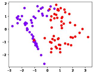
1.建立数据集
class_1_ = 7
class_2_ = 4
centers_ = [[0.0, 0.0], [1,1]]
clusters_std = [0.5, 1]
X_, y_ = make_blobs(n_samples=[class_1_, class_2_],
                  centers=centers_,
                  cluster_std=clusters_std,
                  random_state=0, shuffle=False)#shuffle()将序列的所有元素随机排序
plt.scatter(X_[:, 0], X_[:, 1], c=y_, cmap="rainbow",s=30)
plt.show()

2.建模调用概率
from sklearn.linear_model import LogisticRegression as LogiR
clf_lo = LogiR().fit(X_,y_)
prob = clf_lo.predict_proba(X_)
prob
array([[0.69461879, 0.30538121],
       [0.5109308 , 0.4890692 ],
       [0.82003826, 0.17996174],
       [0.78564706, 0.21435294],
       [0.77738721, 0.22261279],
       [0.65663421, 0.34336579],
       [0.76858638, 0.23141362],
       [0.34917129, 0.65082871],
       [0.36618382, 0.63381618],
       [0.66327186, 0.33672814],
       [0.6075288 , 0.3924712 ]])
prob.shape#代表了十一个样本,的两个数据分别为属于两类的概率
(11, 2)
#将样本和概率放到一个DataFrame中
import pandas as pd
prob = pd.DataFrame(prob)
prob.columns = ["0","1"]#给列取名
prob #似然,属于0或1 的可能性
| 0 | 1 | |
|---|---|---|
| 0 | 0.694619 | 0.305381 |
| 1 | 0.510931 | 0.489069 |
| 2 | 0.820038 | 0.179962 |
| 3 | 0.785647 | 0.214353 |
| 4 | 0.777387 | 0.222613 |
| 5 | 0.656634 | 0.343366 |
| 6 | 0.768586 | 0.231414 |
| 7 | 0.349171 | 0.650829 |
| 8 | 0.366184 | 0.633816 |
| 9 | 0.663272 | 0.336728 |
| 10 | 0.607529 | 0.392471 |
3.使用阈值0.5进行预测分类
#手动调节阈值,来改变我们的模型效果
for i in range(prob.shape[0]):
    if prob.loc[i,"1"] > 0.5:
        prob.loc[i,"pred"] = 1
    else:
        prob.loc[i,"pred"] = 0
prob
| 0 | 1 | pred | |
|---|---|---|---|
| 0 | 0.694619 | 0.305381 | 0.0 |
| 1 | 0.510931 | 0.489069 | 0.0 |
| 2 | 0.820038 | 0.179962 | 0.0 |
| 3 | 0.785647 | 0.214353 | 0.0 |
| 4 | 0.777387 | 0.222613 | 0.0 |
| 5 | 0.656634 | 0.343366 | 0.0 |
| 6 | 0.768586 | 0.231414 | 0.0 |
| 7 | 0.349171 | 0.650829 | 1.0 |
| 8 | 0.366184 | 0.633816 | 1.0 |
| 9 | 0.663272 | 0.336728 | 0.0 |
| 10 | 0.607529 | 0.392471 | 0.0 |
prob["y_true"] = y_
prob = prob.sort_values(by="1",ascending=False)#降序排列,ascending是否倒序
prob
| 0 | 1 | pred | y_true | |
|---|---|---|---|---|
| 7 | 0.349171 | 0.650829 | 1.0 | 1 |
| 8 | 0.366184 | 0.633816 | 1.0 | 1 |
| 1 | 0.510931 | 0.489069 | 0.0 | 0 |
| 10 | 0.607529 | 0.392471 | 0.0 | 1 |
| 5 | 0.656634 | 0.343366 | 0.0 | 0 |
| 9 | 0.663272 | 0.336728 | 0.0 | 1 |
| 0 | 0.694619 | 0.305381 | 0.0 | 0 |
| 6 | 0.768586 | 0.231414 | 0.0 | 0 |
| 4 | 0.777387 | 0.222613 | 0.0 | 0 |
| 3 | 0.785647 | 0.214353 | 0.0 | 0 |
| 2 | 0.820038 | 0.179962 | 0.0 | 0 |
4.使用混淆矩阵查看结果
from sklearn.metrics import confusion_matrix as CM, precision_score as P, recall_score as R
# CM混淆矩阵P精确度,R召回率
CM(prob.loc[:,"y_true"],prob.loc[:,"pred"],labels=[1,0])
#真实值,预测值,少数类标签在前
array([[2, 2],
       [0, 7]], dtype=int64)
#少数类被分类2对,2错,多数类0错,7对
#试试看手动计算Precision和Recall?
2/3
0.6666666666666666
0.5
0.5
P(prob.loc[:,"y_true"],prob.loc[:,"pred"],labels=[1,0])
1.0
R(prob.loc[:,"y_true"],prob.loc[:,"pred"],labels=[1,0])
0.5
5.修改阈值为0.3
for i in range(prob.shape[0]):
    if prob.loc[i,"1"] > 0.3:
        prob.loc[i,"pred"] = 1
    else:
        prob.loc[i,"pred"] = 0
prob
| 0 | 1 | pred | y_true | |
|---|---|---|---|---|
| 7 | 0.349171 | 0.650829 | 1.0 | 1 |
| 8 | 0.366184 | 0.633816 | 1.0 | 1 |
| 1 | 0.510931 | 0.489069 | 1.0 | 0 |
| 10 | 0.607529 | 0.392471 | 1.0 | 1 |
| 5 | 0.656634 | 0.343366 | 1.0 | 0 |
| 9 | 0.663272 | 0.336728 | 1.0 | 1 |
| 0 | 0.694619 | 0.305381 | 1.0 | 0 |
| 6 | 0.768586 | 0.231414 | 0.0 | 0 |
| 4 | 0.777387 | 0.222613 | 0.0 | 0 |
| 3 | 0.785647 | 0.214353 | 0.0 | 0 |
| 2 | 0.820038 | 0.179962 | 0.0 | 0 |
CM(prob.loc[:,"y_true"],prob.loc[:,"pred"],labels=[1,0])
array([[4, 0],
       [3, 4]], dtype=int64)
P(prob.loc[:,"y_true"],prob.loc[:,"pred"],labels=[1,0])
0.5714285714285714
R(prob.loc[:,"y_true"],prob.loc[:,"pred"],labels=[1,0])
1.0
#通常来说,降低阈值能够升高Recall
3.2 置信度参数 decision_function,predict_proba
#使用最初的X和y,样本不均衡的这个模型

class_1 = 500 #类别1有500个样本
class_2 = 50 #类别2只有50个
centers = [[0.0, 0.0], [2.0, 2.0]] #设定两个类别的中心
clusters_std = [1.5, 0.5] #设定两个类别的方差,通常来说,样本量比较大的类别会更加松散
X, y = make_blobs(n_samples=[class_1, class_2],
                  centers=centers,
                  cluster_std=clusters_std,
                  random_state=0, shuffle=False)#shuffle随机排序列表
#看看数据集长什么样
plt.scatter(X[:, 0], X[:, 1], c=y, cmap="rainbow",s=10)
#其中红色点是少数类,紫色点是多数类

clf_proba = svm.SVC(kernel="linear",C=1.0,probability=True).fit(X,y)
#probability这个接口增加运算量,若值并非强制要求0-1分布,就不用了
clf_proba.predict_proba(X)
array([[0.68765639, 0.31234361],
       [0.25911428, 0.74088572],
       [0.96424822, 0.03575178],
       ...,
       [0.1517117 , 0.8482883 ],
       [0.35313082, 0.64686918],
       [0.31213505, 0.68786495]])
clf_proba.predict_proba(X).shape #生成的各类标签下的概率(把置信度强行改为概率 )
(550, 2)
clf_proba.decision_function(X) #点到直线的距离,不被约束在0-1之间
array([ -0.39182241,   0.95617053,  -2.24996184,  -2.63659269,
        -3.65243197,  -1.67311996,  -2.56396417,  -2.80650393,
        -1.76184723,  -4.7948575 ,  -7.59061196,  -3.66174848,
        -2.2508023 ,  -4.27626526,   0.78571364,  -3.24751892,
        -8.57016271,  -4.45823747,  -0.14034183,  -5.20657114,
        -8.02181046,  -4.18420871,  -5.6222409 ,  -5.12602771,
        -7.22592707,  -5.07749638,  -6.72386021,  -3.4945225 ,
        -3.51475144,  -5.72941551,  -5.79160724,  -8.06232013,
        -4.36303857,  -6.25419679,  -5.59426696,  -2.60919281,
        -3.90887478,  -4.38754704,  -6.46432224,  -4.54279979,
        -4.78961735,  -5.53727469,   1.33920817,  -2.27766451,
        -4.39650854,  -2.97649872,  -2.26771979,  -2.40781748,
        -1.41638181,  -3.26142275,  -2.7712218 ,  -4.87288439,
        -3.2594128 ,  -5.91189118,   1.48676267,   0.5389064 ,
        -2.76188843,  -3.36126945,  -2.64697843,  -1.63635284,
        -5.04695135,  -1.59196902,  -5.5195418 ,  -2.10439349,
        -2.29646147,  -4.63162339,  -5.21532213,  -4.19325629,
        -3.37620335,  -5.0032094 ,  -6.04506666,  -2.84656859,
         1.5004014 ,  -4.02677739,  -7.07160609,  -1.66193239,
        -6.60981996,  -5.23458676,  -3.70189918,  -6.74089425,
        -2.09584948,  -2.28398296,  -4.97899921,  -8.12174085,
        -1.52566274,  -1.99176286,  -3.54013094,  -4.8845886 ,
        -6.51002015,  -4.8526957 ,  -6.73649174,  -8.50103589,
        -5.35477446,  -5.93972132,  -3.09197136,  -5.95218482,
        -5.87802088,  -3.41531761,  -1.50581423,   1.69513218,
        -5.08155767,  -1.17971205,  -5.3506946 ,  -5.21493342,
        -3.73358514,  -2.01273566,  -3.39045625,  -6.34357458,
        -3.54776648,  -0.17804673,  -6.26887557,  -4.17973771,
        -6.68896346,  -3.46095619,  -5.47965411,  -7.30835247,
        -4.41569899,  -4.95103272,  -4.52261342,  -2.32912228,
        -5.78601433,  -4.75347157,  -7.10337939,  -0.4589064 ,
        -7.67789856,  -4.01780827,  -4.3031773 ,  -1.83727693,
        -7.40091653,  -5.95271547,  -6.91568411,  -5.20341905,
        -7.19695832,  -3.02927263,  -4.48056922,  -7.48496425,
        -0.07011269,  -5.80292499,  -3.38503533,  -4.58498843,
        -2.76260661,  -3.01843998,  -2.67539002,  -4.1197355 ,
        -0.94129257,  -5.89363772,  -1.6069038 ,  -2.6343464 ,
        -3.04465464,  -4.23219535,  -3.91622593,  -5.29389964,
        -3.59245628,  -8.41452726,  -3.09845691,  -2.71798914,
        -7.1383473 ,  -4.61490324,  -4.57817871,  -4.34638288,
        -6.5457838 ,  -4.91701759,  -6.57235561,  -1.01417607,
        -3.91893483,  -4.52905816,  -4.47582917,  -7.84694737,
        -6.49226452,  -2.82193743,  -2.87607739,  -7.0839848 ,
        -5.2681034 ,  -4.4871544 ,  -2.54658631,  -7.54914279,
        -2.70628288,  -5.99557957,  -8.02076603,  -4.00226228,
        -2.84835501,  -1.9410333 ,  -3.86856886,  -4.99855904,
        -6.21947623,  -5.05797444,  -2.97214824,  -3.26123902,
        -5.27649982,  -3.13897861,  -6.48514315,  -9.55083209,
        -6.46488612,  -7.98793665,  -0.94456569,  -3.41380968,
        -7.093158  ,  -5.71901588,  -0.88438995,  -0.24381463,
        -6.78212695,  -2.20666714,  -6.65580329,  -2.56305221,
        -5.60001636,  -5.43216357,  -4.96741585,  -0.02572912,
        -3.21839147,   1.13383091,  -1.58640099,  -7.57106914,
        -4.16850181,  -6.48179088,  -4.67852158,  -6.99661419,
        -2.1447926 ,  -5.31694653,  -2.63007619,  -2.55890478,
        -6.4896746 ,  -3.94241071,  -2.71319258,  -4.70525843,
        -5.61592746,  -4.7150336 ,  -2.85352156,  -0.49195707,
        -8.16191324,  -3.80462978,  -6.43680611,  -4.58137592,
        -1.38912206,  -6.93900334,  -7.7222725 ,  -8.41592264,
        -5.613998  ,   0.44396046,  -3.07168078,  -1.36478732,
        -1.20153628,  -6.30209808,  -6.49846303,  -0.60518198,
        -3.83301464,  -6.40455571,  -0.22680504,   0.54161373,
        -5.99626181,  -5.98077412,  -3.45857531,  -2.50268554,
        -5.54970836,  -9.26535525,  -4.22097425,  -0.47257602,
        -9.33187038,  -4.97705346,  -1.65256318,  -1.0000177 ,
        -5.82202444,  -8.34541689,  -4.97060946,  -0.34446784,
        -6.95722208,  -7.41413036,  -1.8343221 ,  -7.19145712,
        -4.8082824 ,  -4.59805445,  -5.49449995,  -2.25570223,
        -5.41145249,  -5.97739476,  -2.94240518,  -3.64911853,
        -2.82208944,  -3.34705766,  -8.19712182,  -7.57201089,
        -0.61670956,  -6.3752957 ,  -5.06738146,  -2.54344987,
        -3.28382401,  -5.9927353 ,  -2.87730848,  -3.58324503,
        -7.1488302 ,  -2.63140119,  -8.48092542,  -4.91672751,
        -5.7488116 ,  -3.80044426,  -9.27859326,  -2.475992  ,
        -6.06980518,  -2.90059294,  -5.22496057,  -5.97575155,
        -6.18156775,  -5.38363878,  -7.41985155,  -6.73241325,
        -4.43878791,  -9.06614408,  -1.69153658,  -3.71141045,
        -3.19852116,  -4.05473804,  -3.45821856,  -4.92039492,
        -6.55332449,  -1.28332784,  -4.17989583,  -5.45916562,
        -3.80974949,  -4.27838346,  -5.31607024,  -0.62628865,
        -2.21276478,  -3.7397342 ,  -6.66779473,  -2.38116892,
        -2.83460004,  -7.01238422,  -2.75282445,  -3.01759368,
        -6.14970454,  -6.1300394 ,  -7.58620719,  -3.14051577,
        -5.82720807,  -2.52236034,  -7.03761018,  -7.82753368,
        -8.8447092 ,  -3.11218173,  -4.22074847,  -0.99624534,
        -3.45189404,  -1.46956557,  -9.42857926,  -2.75093993,
        -0.61665367,  -2.09370852,  -9.34768018,  -3.39876535,
        -5.8635608 ,  -2.12987936,  -8.40706474,  -3.84209244,
        -0.5100329 ,  -2.48836494,  -1.54663048,  -4.30920238,
        -5.73107193,  -1.89978615,  -6.17605033,  -3.10487492,
        -5.51376743,  -4.32751131,  -8.20349197,  -3.87477609,
        -1.78392197,  -6.17403966,  -6.52743333,  -3.02302099,
        -4.99201913,  -5.72548424,  -7.83390422,  -1.19722286,
        -4.59974076,  -2.99496132,  -6.83038116,  -5.1842235 ,
        -0.78127198,  -2.88907207,  -3.95055581,  -6.33003274,
        -4.47772201,  -2.77425683,  -4.44937971,  -4.2292366 ,
        -1.15145162,  -4.92325347,  -5.40648383,  -7.37247783,
        -4.65237446,  -7.04281259,  -0.69437244,  -4.99227188,
        -3.02282976,  -2.52532913,  -6.52636286,  -5.48318846,
        -3.71028837,  -6.91757625,  -5.54349414,  -6.05345046,
        -0.43986605,  -4.75951272,  -1.82851406,  -3.24432919,
        -7.20785221,  -4.0583863 ,  -3.27842271,  -0.68706448,
        -2.76021537,  -5.54119808,  -4.08188794,  -6.4244794 ,
        -4.76668274,  -0.2040958 ,  -2.42898945,  -2.03283232,
        -4.12879797,  -2.70459163,  -6.04997273,  -2.79280244,
        -4.20663028,   0.786804  ,  -3.65237777,  -3.55179726,
        -5.3460864 , -10.31959605,  -6.69397854,  -6.53784926,
        -7.56321471,  -4.98085596,  -1.79893146,  -3.89513404,
        -5.18601688,  -3.82352518,  -5.20243998,  -3.11707515,
        -5.80322513,  -4.42380099,  -5.74159836,  -6.6468986 ,
        -3.18053496,  -4.28898663,  -6.73111304,  -3.21485845,
        -4.79047586,  -4.51550728,  -2.70659984,  -3.61545839,
        -7.86496861,  -0.1258212 ,  -7.6559803 ,  -3.15269699,
        -2.87456418,  -6.74876767,  -0.42574712,  -7.58877495,
        -5.30321115,  -4.79881591,  -4.5673199 ,  -3.6865868 ,
        -4.46822682,  -1.45060265,  -0.53560561,  -4.94874171,
        -1.26112294,  -1.66779284,  -5.57910033,  -5.87103484,
        -3.35570045,  -6.25661833,  -1.51564145,   0.85085628,
        -3.82725071,  -1.47077448,  -3.36154118,  -5.37972404,
        -2.22844631,  -2.78684422,  -3.75603932,  -1.85645   ,
        -3.33156093,  -2.32968944,  -5.06053069,  -1.73410541,
        -1.68829408,  -3.79892942,  -1.62650712,  -1.00001873,
        -6.07170511,  -4.89697898,  -3.66269926,  -3.13731451,
        -5.08348781,  -3.71891247,  -2.09779606,  -3.04082162,
        -5.12536015,  -2.96071945,  -4.28796395,  -6.6231135 ,
         1.00003406,   0.03907036,   0.46718521,  -0.3467975 ,
         0.32350521,   0.47563771,   1.10055427,  -0.67580418,
        -0.46310299,   0.40806733,   1.17438632,  -0.55152081,
         0.84476439,  -0.91257798,   0.63165546,  -0.13845693,
        -0.22137683,   1.20116183,   1.18915628,  -0.40676459,
         1.35964325,   1.14038015,   1.27914468,   0.19329823,
        -0.16790648,  -0.62775078,   0.66095617,   2.18236076,
         0.07018415,  -0.26762451,  -0.25529448,   0.32084111,
         0.48016592,   0.28189794,   0.60568093,  -1.07472716,
        -0.5088941 ,   0.74892526,   0.07203056,  -0.10668727,
        -0.15662946,   0.09611498,  -0.39521586,  -0.79874442,
         0.65613691,  -0.39386485,  -1.08601917,   1.44693858,
         0.62992794,   0.76536897])
clf_proba.decision_function(X).shape
(550,)
prob
| 0 | 1 | pred | y_true | |
|---|---|---|---|---|
| 7 | 0.349171 | 0.650829 | 1.0 | 1 |
| 8 | 0.366184 | 0.633816 | 1.0 | 1 |
| 1 | 0.510931 | 0.489069 | 1.0 | 0 |
| 10 | 0.607529 | 0.392471 | 1.0 | 1 |
| 5 | 0.656634 | 0.343366 | 1.0 | 0 |
| 9 | 0.663272 | 0.336728 | 1.0 | 1 |
| 0 | 0.694619 | 0.305381 | 1.0 | 0 |
| 6 | 0.768586 | 0.231414 | 0.0 | 0 |
| 4 | 0.777387 | 0.222613 | 0.0 | 0 |
| 3 | 0.785647 | 0.214353 | 0.0 | 0 |
| 2 | 0.820038 | 0.179962 | 0.0 | 0 |
3.3 绘制SVM的ROC曲线
#从混淆矩阵中获取FPR和Recall
cm = CM(prob.loc[:,"y_true"],prob.loc[:,"pred"],labels=[1,0])
cm
array([[4, 0],
       [3, 4]], dtype=int64)
#00/all true 0 ;1-特异度
#FPR #被我们预测错误的0(真实为0,被预测为1)占所有真正为0的样本的比例
#第0行对应少数类,真实值为1;第一行对应多数类,真实值为0;
#3/(3+4)
cm[1,0]/cm[1,:].sum()
0.42857142857142855
#Recall
#4/(4+0)
cm[0,0]/cm[0,:].sum()
1.0
#概率 clf_proba.predict_proba(X)[:,1] #我的类别1下面的概率
#阈值,每一个阈值都对应着一次循环,每一次循环,都要有一个混淆矩阵,要有一组假正率vsRecall
#np.lispance(概率最小值,概率最大值,55,endpoint=False) #endpoint=False:不要取到最大值,否则无法分为两类
#if i > 概率最大值, 返回1
#开始绘图
probrange = np.linspace(clf_proba.predict_proba(X)[:,1].min(),clf_proba.predict_proba(X)[:,1].max(),num=50,endpoint=False)

from sklearn.metrics import confusion_matrix as CM, recall_score as R
import matplotlib.pyplot as plot

recall = []
FPR = []

for i in probrange:
    y_predict = []
    for j in range(X.shape[0]):
        if clf_proba.predict_proba(X)[j,1] > i:
            y_predict.append(1)
        else:
            y_predict.append(0)
    cm = CM(y,y_predict,labels=[1,0])#labels表示标签为1的是少数类
    recall.append(cm[0,0]/cm[0,:].sum())
    FPR.append(cm[1,0]/cm[1,:].sum())
# 生成每一个阈值底下的混淆矩阵,recall,precision
recall.sort()
FPR.sort()

plt.plot(FPR,recall,c="red")
plt.plot(probrange+0.05,probrange+0.05,c="black",linestyle="--")#y=x的中间线
plt.show()

#x轴precision假正率,越大代表多数类被误判越多
#y轴recall召回率,越大代表捕获越少数类完全

#ROC曲线就是,假正率顺序列表和召回率顺序列表构成的曲线
#我们希望假正率低,召回率高,因此希望曲线趋于左上角弯曲

#当ROC曲线趋于右下角时,说明少数类判断错误,只需要修改少数类标签label即可

#越接近中间的黑线模型越糟糕

3.4 sklearn中ROC与AUC
from sklearn.metrics import roc_curve
FPR, recall, thresholds = roc_curve(y,clf_proba.decision_function(X), pos_label=1)
#真实标签,置信度分数,positive_label正样本标签
FPR.shape
(45,)
recall.shape
(45,)
thresholds.shape #此时的threshold阈值 就不是一个概率值,而是距离值(带方向)中的阈值了,所以它可以大于1,也可以为负
(45,)
thresholds #decision_function
array([  3.18236076,   2.18236076,   1.48676267,   1.35964325,
         1.33920817,   1.14038015,   1.13383091,   1.00003406,
         0.85085628,   0.84476439,   0.78571364,   0.60568093,
         0.5389064 ,   0.46718521,   0.44396046,   0.03907036,
        -0.07011269,  -0.10668727,  -0.1258212 ,  -0.13845693,
        -0.14034183,  -0.16790648,  -0.2040958 ,  -0.22137683,
        -0.24381463,  -0.26762451,  -0.34446784,  -0.3467975 ,
        -0.39182241,  -0.40676459,  -0.4589064 ,  -0.46310299,
        -0.49195707,  -0.5088941 ,  -0.53560561,  -0.55152081,
        -0.62628865,  -0.67580418,  -0.78127198,  -0.79874442,
        -0.88438995,  -0.91257798,  -1.01417607,  -1.08601917,
       -10.31959605])
from sklearn.metrics import roc_auc_score as AUC
AUC(y,clf_proba.decision_function(X))
0.9696400000000001
area = AUC(y,clf_proba.decision_function(X))
#min = 0
#max = 1
plt.figure()
plt.plot(FPR, recall, color='red',
         label='ROC curve (area = %0.2f)' % area)#画标签
plt.plot([0, 1], [0, 1], color='black',linestyle='--')#画一条0-1之间的虚线
plt.xlim([-0.05, 1.05])
plt.ylim([-0.05, 1.05])
plt.xlabel('False Positive Rate')
plt.ylabel('Recall')
plt.title('Receiver operating characteristic example')
plt.legend(loc="lower right")#显示图例显示在右下脚
plt.show()

3.5 利用ROC曲线寻找最佳阈值
max((recall - FPR).tolist())
0.914
#lits.index(最大值) #返回这个最大值在list中的索引
(recall-FPR)
array([0.   , 0.02 , 0.014, 0.054, 0.052, 0.152, 0.15 , 0.19 , 0.186,
       0.206, 0.202, 0.342, 0.338, 0.398, 0.396, 0.576, 0.572, 0.592,
       0.59 , 0.61 , 0.608, 0.648, 0.644, 0.664, 0.66 , 0.7  , 0.698,
       0.718, 0.716, 0.776, 0.77 , 0.79 , 0.786, 0.806, 0.802, 0.822,
       0.814, 0.854, 0.848, 0.868, 0.866, 0.886, 0.874, 0.914, 0.   ])
maxindex = (recall - FPR).tolist().index(max(recall - FPR))
maxindex #recall, FPR
43
thresholds[maxindex] #decision_function生成的置信度来说对应的最佳阈值
-1.0860191749391461
#我们可以在图像上来看看这个点在哪里
plt.scatter(FPR[maxindex],recall[maxindex],c="black",s=30)

#把上述代码放入这段代码中:
plt.figure()
plt.plot(FPR, recall, color='red',
         label='ROC curve (area = %0.2f)' % area)
plt.plot([0, 1], [0, 1], color='black', linestyle='--')
plt.scatter(FPR[maxindex],recall[maxindex],c="black",s=30)#离左上角最近的点,离中间黑色分割线最远的点
plt.xlim([-0.05, 1.05])
plt.ylim([-0.05, 1.05])
plt.xlabel('False Positive Rate')
plt.ylabel('Recall')
plt.title('Receiver operating characteristic example')
plt.legend(loc="lower right")
plt.show()

clf_proba.dual_coef_ #查看生成的拉格朗日乘子
array([[-1.        , -1.        , -1.        , -1.        , -1.        ,
        -1.        , -1.        , -1.        , -1.        , -1.        ,
        -1.        , -1.        , -1.        , -1.        , -1.        ,
        -1.        , -1.        , -1.        , -1.        , -1.        ,
        -1.        , -1.        , -1.        , -1.        , -0.50312301,
        -1.        , -1.        , -1.        , -1.        , -1.        ,
        -1.        , -1.        , -1.        , -1.        , -1.        ,
        -1.        , -1.        , -1.        , -1.        , -1.        ,
        -1.        , -0.25015141,  0.75327442,  1.        ,  1.        ,
         1.        ,  1.        ,  1.        ,  1.        ,  1.        ,
         1.        ,  1.        ,  1.        ,  1.        ,  1.        ,
         1.        ,  1.        ,  1.        ,  1.        ,  1.        ,
         1.        ,  1.        ,  1.        ,  1.        ,  1.        ,
         1.        ,  1.        ,  1.        ,  1.        ,  1.        ,
         1.        ,  1.        ,  1.        ,  1.        ,  1.        ,
         1.        ,  1.        ,  1.        ,  1.        ,  1.        ,
         1.        ,  1.        ,  1.        ]])
clf_proba.support_vectors_.shape#查看支持向量属性
(83, 2)
clf_proba.dual_coef_.shape
(1, 83)