sklearn_Lasso与多项式回归_菜菜视频学习笔记
lasso与多项式回归
- 1 Lasso与多重共线性
-
- 1.1 Lasso 强大的特征选择能力
- 1.2 选取最佳正则化参数
- 2. 非线性问题:多项式回归
-
- 2.1 使用分箱处理非线性问题
- 2.2多项式回归PolynomialFeatures
-
- 2.2.1多项式对数据的作用
- 2.2.2 多项式回归如何处理非线性问题
- 2.2.3 多项式回归的可解释性
1 Lasso与多重共线性
# Lasso与多重共线性
#Lasso 全称为最小绝对收缩和选择算子
# Lasso 的正则项是系数为w的L1范式*系数α
# L1范式所带的正则项α在求导后不带有w这个项,它无法对(X^T)X矩阵造成影响,lasso无法解决特征之间的“精确相关问题”问题
# 当我们使用最小二乘法解决线性回归问题时,如果线性回归无解或报除零错误,换Lasso无法解决问题,而岭回归可以

# 当多重共线性问题只是"高度相关",我们方阵(X^T)X的逆存在
# 等式两边乘以方阵的逆后,通过增大α来增加一个负项,来控制方阵左边式子的大小使其接近与0,得以调节方阵过大对w的影响
# 防止参数w过大,对导致模型失准问题
# Lasso不是从根本上解决多重共线性问题,而是限制了多重共线性带来的影响
# (以上为所有系数都为正的情况,当系数w非正,可能需要把正则化参数设定为负数,且负数越大,对共线性的影响越大)
1.1 Lasso 强大的特征选择能力
# Lasso 强大的特征选择能力
# L1正则化主导稀疏性,会将系数压缩到0,这个特性让lasso成为特征选择工具的首选
# Lasso(positive),当参数positice为真时,Lasso返回的系数就必须是正数,来确保α是通过增大来控制正则化程度


import numpy as np
import pandas as pd
from sklearn.linear_model import Ridge, LinearRegression, Lasso
from sklearn.model_selection import train_test_split as TTS
from sklearn.datasets import fetch_california_housing as fch
import matplotlib.pyplot as plt

housevalue = fch()

X = pd.DataFrame(housevalue.data)
y = housevalue.target
X.columns = ["住户收入中位数","房屋使用年代中位数","平均房间数目"
            ,"平均卧室数目","街区人口","平均入住率","街区的纬度","街区的经度"]

X.head()
| 住户收入中位数 | 房屋使用年代中位数 | 平均房间数目 | 平均卧室数目 | 街区人口 | 平均入住率 | 街区的纬度 | 街区的经度 | |
|---|---|---|---|---|---|---|---|---|
| 0 | 8.3252 | 41.0 | 6.984127 | 1.023810 | 322.0 | 2.555556 | 37.88 | -122.23 |
| 1 | 8.3014 | 21.0 | 6.238137 | 0.971880 | 2401.0 | 2.109842 | 37.86 | -122.22 |
| 2 | 7.2574 | 52.0 | 8.288136 | 1.073446 | 496.0 | 2.802260 | 37.85 | -122.24 |
| 3 | 5.6431 | 52.0 | 5.817352 | 1.073059 | 558.0 | 2.547945 | 37.85 | -122.25 |
| 4 | 3.8462 | 52.0 | 6.281853 | 1.081081 | 565.0 | 2.181467 | 37.85 | -122.25 |
Xtrain,Xtest,Ytrain,Ytest = TTS(X,y,test_size=0.3,random_state=420)
for i in [Xtrain,Xtest]:
    i.index = range(i.shape[0])
#线性回归进行拟合
reg = LinearRegression().fit(Xtrain,Ytrain)
(reg.coef_*100).tolist()
[43.735893059684074,
 1.0211268294494147,
 -10.780721617317637,
 62.64338275363747,
 5.21612535296645e-05,
 -0.33485096463334924,
 -41.30959378947715,
 -42.62109536208473]
#岭回归进行拟合
Ridge_ = Ridge(alpha=0).fit(Xtrain,Ytrain)
(Ridge_.coef_*100).tolist()
[43.73589305968356,
 1.0211268294493694,
 -10.780721617316962,
 62.6433827536353,
 5.2161253532548055e-05,
 -0.3348509646333529,
 -41.30959378947995,
 -42.62109536208777]
#Lasso进行拟合
lasso_ = Lasso(alpha=0).fit(Xtrain,Ytrain)
(lasso_.coef_*100).tolist()
# 岭回归,lasso与线性回归结果几乎没什么不同

# Lasso正则化系数为0,算法不可收敛

# Lasso 使用的是坐标下降法求解,没有正则化,可能导致意外结果

# 目标没有收敛。您可能希望增加迭代次数。用非常小的 alpha 拟合数据可能会导致精度问题。
C:\Users\chen'bu'rong\AppData\Local\Temp\ipykernel_17824\3627946873.py:2: UserWarning: With alpha=0, this algorithm does not converge well. You are advised to use the LinearRegression estimator
  lasso_ = Lasso(alpha=0).fit(Xtrain,Ytrain)
D:\py1.1\lib\site-packages\sklearn\linear_model\_coordinate_descent.py:648: UserWarning: Coordinate descent with no regularization may lead to unexpected results and is discouraged.
  model = cd_fast.enet_coordinate_descent(
D:\py1.1\lib\site-packages\sklearn\linear_model\_coordinate_descent.py:648: ConvergenceWarning: Objective did not converge. You might want to increase the number of iterations, check the scale of the features or consider increasing regularisation. Duality gap: 3.770e+03, tolerance: 1.917e+00 Linear regression models with null weight for the l1 regularization term are more efficiently fitted using one of the solvers implemented in sklearn.linear_model.Ridge/RidgeCV instead.
  model = cd_fast.enet_coordinate_descent(


[43.73589305968407,
 1.0211268294494082,
 -10.780721617317662,
 62.6433827536377,
 5.21612535327013e-05,
 -0.33485096463335806,
 -41.30959378947693,
 -42.621095362084496]
#岭回归进行拟合
Ridge_ = Ridge(alpha=0.1).fit(Xtrain,Ytrain)
(Ridge_.coef_*100).tolist()
[43.734534807869196,
 1.0211508518425259,
 -10.778109335481327,
 62.62978997580269,
 5.2255520319229976e-05,
 -0.3348478363544321,
 -41.3093700653905,
 -42.62068050768773]
#Lasso进行拟合
# Lasso的alpha系数异常敏感
lasso_ = Lasso(alpha=0.1).fit(Xtrain,Ytrain)
(lasso_.coef_*100).tolist()
[39.08851438329682,
 1.6054695654279867,
 -0.0,
 0.0,
 0.0023777014839091335,
 -0.3050186895638112,
 -10.771509301655538,
 -9.294344477958074]
[43.73589305968403,
 1.0211268294494038,
 -10.780721617317715,
 62.64338275363783,
 5.216125353178735e-05,
 -0.33485096463336095,
 -41.30959378947711,
 -42.621095362084674]
[43.73589305968403,
 1.0211268294494038,
 -10.780721617317715,
 62.64338275363783,
 5.216125353178735e-05,
 -0.33485096463336095,
 -41.30959378947711,
 -42.621095362084674]
#加大正则项系数,观察模型的系数发生了什么变化
Ridge_ = Ridge(alpha=10**10).fit(Xtrain,Ytrain)
(Ridge_.coef_*100).tolist()
# 即使alpha再大,参数值也取不到0
[0.00021838533330206371,
 0.00021344956264503437,
 6.213673042878628e-05,
 -3.828084920732722e-06,
 -0.001498408728695283,
 -4.175243714653839e-05,
 -5.295061194474971e-05,
 -1.3268982521957738e-05]
#加大正则项系数,观察模型的系数发生了什么变化
Ridge_ = Ridge(alpha=10**4).fit(Xtrain,Ytrain)
(Ridge_.coef_*100).tolist()
[34.62081517607707,
 1.5196170869238759,
 0.3968610529209999,
 0.915181251035547,
 0.0021739238012248533,
 -0.34768660148101127,
 -14.73696347421548,
 -13.435576102527182]
lasso_ = Lasso(alpha=10**4).fit(Xtrain,Ytrain)
(lasso_.coef_*100).tolist()
[0.0, 0.0, 0.0, -0.0, -0.0, -0.0, -0.0, -0.0]
#看来10**4对于Lasso来说是一个过于大的取值
lasso_ = Lasso(alpha=1).fit(Xtrain,Ytrain)
(lasso_.coef_*100).tolist()
# 证明Lasso对alpha系数的极度敏感
# 特征选择:去掉那些w参数为0的特征
[14.581141247629409,
 0.6209347344423877,
 0.0,
 -0.0,
 -0.0002806598632900984,
 -0.0,
 -0.0,
 -0.0]
#将系数进行绘图
plt.plot(range(1,9),(reg.coef_*100).tolist(),color="red",label="LR")
plt.plot(range(1,9),(Ridge_.coef_*100).tolist(),color="orange",label="Ridge")
plt.plot(range(1,9),(lasso_.coef_*100).tolist(),color="k",label="Lasso")
plt.plot(range(1,9),[0]*8,color="grey",linestyle="--")
plt.xlabel('w') #横坐标是每一个特征所对应的系数
plt.legend()
plt.show()

1.2 选取最佳正则化参数
# 选取最佳正则化参数
# alpha参数过于敏感,需要在极小范围内变动
# 参数
# 给定eps正则化路径的长度和n_alphas正则化路径的个数,自动生成一组非常小的α
# alphas 默认为none,使用eps和n_alphas生成alphas取值
# cv  默认三折,LassoCV选用的是均方误差,岭回归的指标自己设定,默认为R^2

# 属性
# alpha_ 调用最佳alpha
# alphas_ 调用所有使用的参数alpha
# mse_path 返回所有交叉验证的结果细节
# coef_ 调用最佳正则化参数下建立模型的系数

from sklearn.linear_model import LassoCV

#自己建立Lasso进行alpha选择的范围
alpharange = np.logspace(-10, -2, 200,base=10)

#其实是形成10为底的指数函数
#10**(-10)到10**(-2)次方

alpharange
array([1.00000000e-10, 1.09698580e-10, 1.20337784e-10, 1.32008840e-10,
       1.44811823e-10, 1.58856513e-10, 1.74263339e-10, 1.91164408e-10,
       2.09704640e-10, 2.30043012e-10, 2.52353917e-10, 2.76828663e-10,
       3.03677112e-10, 3.33129479e-10, 3.65438307e-10, 4.00880633e-10,
       4.39760361e-10, 4.82410870e-10, 5.29197874e-10, 5.80522552e-10,
       6.36824994e-10, 6.98587975e-10, 7.66341087e-10, 8.40665289e-10,
       9.22197882e-10, 1.01163798e-09, 1.10975250e-09, 1.21738273e-09,
       1.33545156e-09, 1.46497140e-09, 1.60705282e-09, 1.76291412e-09,
       1.93389175e-09, 2.12145178e-09, 2.32720248e-09, 2.55290807e-09,
       2.80050389e-09, 3.07211300e-09, 3.37006433e-09, 3.69691271e-09,
       4.05546074e-09, 4.44878283e-09, 4.88025158e-09, 5.35356668e-09,
       5.87278661e-09, 6.44236351e-09, 7.06718127e-09, 7.75259749e-09,
       8.50448934e-09, 9.32930403e-09, 1.02341140e-08, 1.12266777e-08,
       1.23155060e-08, 1.35099352e-08, 1.48202071e-08, 1.62575567e-08,
       1.78343088e-08, 1.95639834e-08, 2.14614120e-08, 2.35428641e-08,
       2.58261876e-08, 2.83309610e-08, 3.10786619e-08, 3.40928507e-08,
       3.73993730e-08, 4.10265811e-08, 4.50055768e-08, 4.93704785e-08,
       5.41587138e-08, 5.94113398e-08, 6.51733960e-08, 7.14942899e-08,
       7.84282206e-08, 8.60346442e-08, 9.43787828e-08, 1.03532184e-07,
       1.13573336e-07, 1.24588336e-07, 1.36671636e-07, 1.49926843e-07,
       1.64467618e-07, 1.80418641e-07, 1.97916687e-07, 2.17111795e-07,
       2.38168555e-07, 2.61267523e-07, 2.86606762e-07, 3.14403547e-07,
       3.44896226e-07, 3.78346262e-07, 4.15040476e-07, 4.55293507e-07,
       4.99450512e-07, 5.47890118e-07, 6.01027678e-07, 6.59318827e-07,
       7.23263390e-07, 7.93409667e-07, 8.70359136e-07, 9.54771611e-07,
       1.04737090e-06, 1.14895100e-06, 1.26038293e-06, 1.38262217e-06,
       1.51671689e-06, 1.66381689e-06, 1.82518349e-06, 2.00220037e-06,
       2.19638537e-06, 2.40940356e-06, 2.64308149e-06, 2.89942285e-06,
       3.18062569e-06, 3.48910121e-06, 3.82749448e-06, 4.19870708e-06,
       4.60592204e-06, 5.05263107e-06, 5.54266452e-06, 6.08022426e-06,
       6.66991966e-06, 7.31680714e-06, 8.02643352e-06, 8.80488358e-06,
       9.65883224e-06, 1.05956018e-05, 1.16232247e-05, 1.27505124e-05,
       1.39871310e-05, 1.53436841e-05, 1.68318035e-05, 1.84642494e-05,
       2.02550194e-05, 2.22194686e-05, 2.43744415e-05, 2.67384162e-05,
       2.93316628e-05, 3.21764175e-05, 3.52970730e-05, 3.87203878e-05,
       4.24757155e-05, 4.65952567e-05, 5.11143348e-05, 5.60716994e-05,
       6.15098579e-05, 6.74754405e-05, 7.40196000e-05, 8.11984499e-05,
       8.90735464e-05, 9.77124154e-05, 1.07189132e-04, 1.17584955e-04,
       1.28989026e-04, 1.41499130e-04, 1.55222536e-04, 1.70276917e-04,
       1.86791360e-04, 2.04907469e-04, 2.24780583e-04, 2.46581108e-04,
       2.70495973e-04, 2.96730241e-04, 3.25508860e-04, 3.57078596e-04,
       3.91710149e-04, 4.29700470e-04, 4.71375313e-04, 5.17092024e-04,
       5.67242607e-04, 6.22257084e-04, 6.82607183e-04, 7.48810386e-04,
       8.21434358e-04, 9.01101825e-04, 9.88495905e-04, 1.08436597e-03,
       1.18953407e-03, 1.30490198e-03, 1.43145894e-03, 1.57029012e-03,
       1.72258597e-03, 1.88965234e-03, 2.07292178e-03, 2.27396575e-03,
       2.49450814e-03, 2.73644000e-03, 3.00183581e-03, 3.29297126e-03,
       3.61234270e-03, 3.96268864e-03, 4.34701316e-03, 4.76861170e-03,
       5.23109931e-03, 5.73844165e-03, 6.29498899e-03, 6.90551352e-03,
       7.57525026e-03, 8.30994195e-03, 9.11588830e-03, 1.00000000e-02])
alpharange.shape
(200,)
Xtrain.head()
| 住户收入中位数 | 房屋使用年代中位数 | 平均房间数目 | 平均卧室数目 | 街区人口 | 平均入住率 | 街区的纬度 | 街区的经度 | |
|---|---|---|---|---|---|---|---|---|
| 0 | 4.1776 | 35.0 | 4.425172 | 1.030683 | 5380.0 | 3.368817 | 37.48 | -122.19 |
| 1 | 5.3261 | 38.0 | 6.267516 | 1.089172 | 429.0 | 2.732484 | 37.53 | -122.30 |
| 2 | 1.9439 | 26.0 | 5.768977 | 1.141914 | 891.0 | 2.940594 | 36.02 | -119.08 |
| 3 | 2.5000 | 22.0 | 4.916000 | 1.012000 | 733.0 | 2.932000 | 38.57 | -121.31 |
| 4 | 3.8250 | 34.0 | 5.036765 | 1.098039 | 1134.0 | 2.779412 | 33.91 | -118.35 |
lasso_ = LassoCV(alphas=alpharange #自行输入的alpha的取值范围
                ,cv=5 #交叉验证的折数
                ).fit(Xtrain, Ytrain)
#查看被选择出来的最佳正则化系数
lasso_.alpha_
0.0020729217795953697
#调用所有交叉验证的结果
lasso_.mse_path_
array([[0.52454913, 0.49856261, 0.55984312, 0.50526576, 0.55262557],
       [0.52361933, 0.49748809, 0.55887637, 0.50429373, 0.55283734],
       [0.52281927, 0.49655113, 0.55803797, 0.5034594 , 0.55320522],
       [0.52213811, 0.49574741, 0.55731858, 0.50274517, 0.55367515],
       [0.52155715, 0.49505688, 0.55669995, 0.50213252, 0.55421553],
       [0.52106069, 0.49446226, 0.55616707, 0.50160604, 0.55480104],
       [0.5206358 , 0.49394903, 0.55570702, 0.50115266, 0.55541214],
       [0.52027135, 0.49350539, 0.55530895, 0.50076146, 0.55603333],
       [0.51995825, 0.49312085, 0.5549639 , 0.50042318, 0.55665306],
       [0.5196886 , 0.49278705, 0.55466406, 0.50013007, 0.55726225],
       [0.51945602, 0.49249647, 0.55440306, 0.49987554, 0.55785451],
       [0.51925489, 0.49224316, 0.55417527, 0.49965404, 0.55842496],
       [0.51908068, 0.49202169, 0.55397615, 0.49946088, 0.55897049],
       [0.51892938, 0.49182782, 0.55380162, 0.49929206, 0.55948886],
       [0.51879778, 0.49165759, 0.55364841, 0.49914421, 0.55997905],
       [0.51868299, 0.49150788, 0.55351357, 0.49901446, 0.5604405 ],
       [0.51858268, 0.49137604, 0.55339469, 0.49890035, 0.56087323],
       [0.51849488, 0.49125956, 0.55328972, 0.4987998 , 0.56127784],
       [0.5184178 , 0.49115652, 0.55319678, 0.49871101, 0.56165507],
       [0.51835002, 0.49106526, 0.55311438, 0.49863248, 0.5620059 ],
       [0.51829033, 0.49098418, 0.55304118, 0.49856287, 0.56233145],
       [0.51823761, 0.49091208, 0.55297609, 0.49850108, 0.56263308],
       [0.51819098, 0.49084785, 0.55291806, 0.49844612, 0.56291204],
       [0.51814966, 0.49079058, 0.55286626, 0.49839716, 0.56316966],
       [0.51811298, 0.49073937, 0.55281996, 0.49835348, 0.56340721],
       [0.51808038, 0.49069355, 0.55277854, 0.49831445, 0.5636261 ],
       [0.51805132, 0.49065249, 0.5527414 , 0.49827953, 0.56382754],
       [0.5180254 , 0.49061566, 0.55270806, 0.49824828, 0.56401276],
       [0.51800224, 0.49058258, 0.55267812, 0.49822015, 0.56418292],
       [0.51798152, 0.49055285, 0.55265118, 0.49819493, 0.56433912],
       [0.51796296, 0.49052608, 0.55262693, 0.49817225, 0.56448243],
       [0.5179463 , 0.49050195, 0.55260507, 0.49815185, 0.56461379],
       [0.51793135, 0.49048019, 0.55258536, 0.49813345, 0.5647342 ],
       [0.51791791, 0.49046055, 0.55256757, 0.49811687, 0.56484448],
       [0.5179058 , 0.49044281, 0.55255149, 0.4981019 , 0.56494544],
       [0.5178949 , 0.49042677, 0.55253695, 0.49808838, 0.56503784],
       [0.51788506, 0.49041226, 0.55252379, 0.49807615, 0.56512236],
       [0.51787619, 0.49039913, 0.55251189, 0.4980651 , 0.56519967],
       [0.51786817, 0.49038724, 0.5525011 , 0.49805509, 0.56527034],
       [0.51786092, 0.49037646, 0.55249132, 0.49804603, 0.56533494],
       [0.51785437, 0.49036669, 0.55248246, 0.49803782, 0.56539397],
       [0.51784843, 0.49035783, 0.55247442, 0.49803037, 0.5654479 ],
       [0.51784306, 0.49034979, 0.55246712, 0.49802362, 0.56549716],
       [0.51783819, 0.49034249, 0.5524605 , 0.49801749, 0.56554215],
       [0.51783377, 0.49033586, 0.55245448, 0.49801193, 0.56558322],
       [0.51782977, 0.49032984, 0.55244901, 0.49800688, 0.56562073],
       [0.51782614, 0.49032437, 0.55244405, 0.49800229, 0.56565496],
       [0.51782284, 0.49031939, 0.55243953, 0.49799812, 0.56568621],
       [0.51781984, 0.49031487, 0.55243543, 0.49799434, 0.56571472],
       [0.51781712, 0.49031076, 0.55243169, 0.49799089, 0.56574074],
       [0.51781465, 0.49030702, 0.5524283 , 0.49798776, 0.56576449],
       [0.5178124 , 0.49030362, 0.55242521, 0.49798491, 0.56578615],
       [0.51781036, 0.49030052, 0.5524224 , 0.49798232, 0.56580591],
       [0.5178085 , 0.4902977 , 0.55241984, 0.49797996, 0.56582394],
       [0.51780681, 0.49029514, 0.55241751, 0.49797781, 0.56584039],
       [0.51780528, 0.4902928 , 0.55241539, 0.49797586, 0.56585539],
       [0.51780388, 0.49029068, 0.55241346, 0.49797408, 0.56586907],
       [0.51780261, 0.49028874, 0.55241171, 0.49797246, 0.56588155],
       [0.51780145, 0.49028698, 0.55241011, 0.49797099, 0.56589293],
       [0.51780039, 0.49028538, 0.55240865, 0.49796965, 0.56590331],
       [0.51779943, 0.49028392, 0.55240732, 0.49796843, 0.56591277],
       [0.51779856, 0.49028258, 0.55240611, 0.49796731, 0.5659214 ],
       [0.51779777, 0.49028137, 0.55240501, 0.4979663 , 0.56592927],
       [0.51779704, 0.49028027, 0.55240401, 0.49796538, 0.56593645],
       [0.51779638, 0.49027926, 0.5524031 , 0.49796454, 0.56594299],
       [0.51779578, 0.49027834, 0.55240226, 0.49796377, 0.56594896],
       [0.51779523, 0.49027751, 0.55240151, 0.49796307, 0.5659544 ],
       [0.51779473, 0.49027675, 0.55240081, 0.49796243, 0.56595936],
       [0.51779428, 0.49027605, 0.55240018, 0.49796185, 0.56596388],
       [0.51779386, 0.49027542, 0.55239961, 0.49796133, 0.565968  ],
       [0.51779349, 0.49027485, 0.55239909, 0.49796085, 0.56597176],
       [0.51779314, 0.49027432, 0.55239861, 0.49796041, 0.56597519],
       [0.51779283, 0.49027384, 0.55239818, 0.49796001, 0.56597831],
       [0.51779254, 0.49027341, 0.55239778, 0.49795964, 0.56598116],
       [0.51779228, 0.49027301, 0.55239742, 0.49795931, 0.56598376],
       [0.51779205, 0.49027265, 0.55239709, 0.49795901, 0.56598613],
       [0.51779183, 0.49027232, 0.55239679, 0.49795873, 0.56598828],
       [0.51779163, 0.49027202, 0.55239652, 0.49795848, 0.56599025],
       [0.51779146, 0.49027174, 0.55239627, 0.49795825, 0.56599205],
       [0.51779129, 0.49027149, 0.55239604, 0.49795804, 0.56599368],
       [0.51779114, 0.49027127, 0.55239584, 0.49795785, 0.56599517],
       [0.51779101, 0.49027106, 0.55239565, 0.49795768, 0.56599653],
       [0.51779088, 0.49027087, 0.55239548, 0.49795752, 0.56599777],
       [0.51779077, 0.4902707 , 0.55239532, 0.49795738, 0.5659989 ],
       [0.51779067, 0.49027054, 0.55239518, 0.49795725, 0.56599993],
       [0.51779057, 0.4902704 , 0.55239505, 0.49795713, 0.56600087],
       [0.51779049, 0.49027027, 0.55239493, 0.49795702, 0.56600172],
       [0.51779041, 0.49027015, 0.55239482, 0.49795692, 0.5660025 ],
       [0.51779034, 0.49027004, 0.55239472, 0.49795683, 0.56600322],
       [0.51779027, 0.49026994, 0.55239463, 0.49795675, 0.56600386],
       [0.51779022, 0.49026985, 0.55239455, 0.49795667, 0.56600446],
       [0.51779016, 0.49026977, 0.55239448, 0.4979566 , 0.56600499],
       [0.51779011, 0.49026969, 0.55239441, 0.49795654, 0.56600549],
       [0.51779007, 0.49026962, 0.55239435, 0.49795648, 0.56600593],
       [0.51779003, 0.49026956, 0.55239429, 0.49795643, 0.56600634],
       [0.51778999, 0.49026951, 0.55239424, 0.49795638, 0.56600671],
       [0.51778996, 0.49026945, 0.55239419, 0.49795634, 0.56600705],
       [0.51778993, 0.49026941, 0.55239415, 0.4979563 , 0.56600736],
       [0.5177899 , 0.49026936, 0.55239411, 0.49795626, 0.56600764],
       [0.51778987, 0.49026932, 0.55239407, 0.49795623, 0.5660079 ],
       [0.51778985, 0.49026929, 0.55239404, 0.4979562 , 0.56600813],
       [0.51778983, 0.49026926, 0.55239401, 0.49795617, 0.56600835],
       [0.51778981, 0.49026923, 0.55239398, 0.49795615, 0.56600854],
       [0.51778979, 0.4902692 , 0.55239396, 0.49795613, 0.56600872],
       [0.51778977, 0.49026918, 0.55239394, 0.49795611, 0.56600888],
       [0.51778976, 0.49026915, 0.55239392, 0.49795609, 0.56600903],
       [0.51778975, 0.49026913, 0.5523939 , 0.49795607, 0.56600916],
       [0.51778973, 0.49026911, 0.55239388, 0.49795605, 0.56600929],
       [0.51778972, 0.4902691 , 0.55239387, 0.49795604, 0.5660094 ],
       [0.51778971, 0.49026908, 0.55239385, 0.49795603, 0.5660095 ],
       [0.5177897 , 0.49026907, 0.55239384, 0.49795602, 0.56600959],
       [0.5177897 , 0.49026905, 0.55239383, 0.49795601, 0.56600968],
       [0.51778969, 0.49026904, 0.55239382, 0.497956  , 0.56600975],
       [0.51778968, 0.49026903, 0.55239381, 0.49795599, 0.56600983],
       [0.51778967, 0.49026902, 0.5523938 , 0.49795598, 0.56600989],
       [0.51778967, 0.49026901, 0.55239379, 0.49795597, 0.56600995],
       [0.51778966, 0.490269  , 0.55239378, 0.49795596, 0.56601   ],
       [0.51778966, 0.490269  , 0.55239378, 0.49795596, 0.56601005],
       [0.51778965, 0.49026899, 0.55239377, 0.49795595, 0.56601009],
       [0.51778965, 0.49026898, 0.55239376, 0.49795595, 0.56601013],
       [0.51778965, 0.49026898, 0.55239376, 0.49795594, 0.56601017],
       [0.51778964, 0.49026897, 0.55239375, 0.49795594, 0.5660102 ],
       [0.51778964, 0.49026897, 0.55239375, 0.49795593, 0.56601023],
       [0.51778964, 0.49026896, 0.55239375, 0.49795593, 0.56601026],
       [0.51778963, 0.49026896, 0.55239374, 0.49795593, 0.56601029],
       [0.51778963, 0.49026896, 0.55239374, 0.49795592, 0.56601031],
       [0.51778963, 0.49026895, 0.55239374, 0.49795592, 0.56601033],
       [0.51778963, 0.49026895, 0.55239373, 0.49795592, 0.56601035],
       [0.51778963, 0.49026895, 0.55239373, 0.49795592, 0.56601037],
       [0.51778962, 0.49026895, 0.55239373, 0.49795591, 0.56601039],
       [0.51778962, 0.49026894, 0.55239373, 0.49795591, 0.5660104 ],
       [0.51778962, 0.49026894, 0.55239372, 0.49795591, 0.56601041],
       [0.51778962, 0.49026894, 0.55239372, 0.49795591, 0.56601043],
       [0.51778962, 0.49026894, 0.55239372, 0.49795591, 0.56601044],
       [0.51778962, 0.49026894, 0.55239372, 0.49795591, 0.56601045],
       [0.51778962, 0.49026894, 0.55239372, 0.49795591, 0.56601046],
       [0.51778962, 0.49026893, 0.55239372, 0.4979559 , 0.56601046],
       [0.51778962, 0.49026893, 0.55239372, 0.4979559 , 0.56601047],
       [0.51778962, 0.49026893, 0.55239372, 0.4979559 , 0.56601048],
       [0.51778961, 0.49026893, 0.55239371, 0.4979559 , 0.56601048],
       [0.51778961, 0.49026893, 0.55239371, 0.4979559 , 0.56601049],
       [0.51778961, 0.49026893, 0.55239371, 0.4979559 , 0.5660105 ],
       [0.51778961, 0.49026893, 0.55239371, 0.4979559 , 0.5660105 ],
       [0.51778961, 0.49026893, 0.55239371, 0.4979559 , 0.5660105 ],
       [0.51778961, 0.49026893, 0.55239371, 0.4979559 , 0.56601051],
       [0.51778961, 0.49026893, 0.55239371, 0.4979559 , 0.56601051],
       [0.51778961, 0.49026893, 0.55239371, 0.4979559 , 0.56601052],
       [0.51778961, 0.49026893, 0.55239371, 0.4979559 , 0.56601052],
       [0.51778961, 0.49026893, 0.55239371, 0.4979559 , 0.56601052],
       [0.51778961, 0.49026892, 0.55239371, 0.4979559 , 0.56601052],
       [0.51778961, 0.49026892, 0.55239371, 0.4979559 , 0.56601053],
       [0.51778961, 0.49026892, 0.55239371, 0.4979559 , 0.56601053],
       [0.51778961, 0.49026892, 0.55239371, 0.4979559 , 0.56601053],
       [0.51778961, 0.49026892, 0.55239371, 0.4979559 , 0.56601053],
       [0.51778961, 0.49026892, 0.55239371, 0.4979559 , 0.56601053],
       [0.51778961, 0.49026892, 0.55239371, 0.4979559 , 0.56601054],
       [0.51778961, 0.49026892, 0.55239371, 0.4979559 , 0.56601054],
       [0.51778961, 0.49026892, 0.55239371, 0.4979559 , 0.56601054],
       [0.51778961, 0.49026892, 0.55239371, 0.4979559 , 0.56601054],
       [0.51778961, 0.49026892, 0.55239371, 0.4979559 , 0.56601054],
       [0.51778961, 0.49026892, 0.55239371, 0.4979559 , 0.56601054],
       [0.51778961, 0.49026892, 0.55239371, 0.4979559 , 0.56601054],
       [0.51778961, 0.49026892, 0.55239371, 0.49795589, 0.56601054],
       [0.51778961, 0.49026892, 0.55239371, 0.49795589, 0.56601054],
       [0.51778961, 0.49026892, 0.55239371, 0.49795589, 0.56601054],
       [0.51778961, 0.49026892, 0.55239371, 0.49795589, 0.56601054],
       [0.51778961, 0.49026892, 0.55239371, 0.49795589, 0.56601054],
       [0.51778961, 0.49026892, 0.55239371, 0.49795589, 0.56601055],
       [0.51778961, 0.49026892, 0.55239371, 0.49795589, 0.56601055],
       [0.51778961, 0.49026892, 0.55239371, 0.49795589, 0.56601055],
       [0.51778961, 0.49026892, 0.55239371, 0.49795589, 0.56601055],
       [0.51778961, 0.49026892, 0.55239371, 0.49795589, 0.56601055],
       [0.51778961, 0.49026892, 0.55239371, 0.49795589, 0.56601055],
       [0.51778961, 0.49026892, 0.55239371, 0.49795589, 0.56601055],
       [0.51778961, 0.49026892, 0.55239371, 0.49795589, 0.56601055],
       [0.51778961, 0.49026892, 0.55239371, 0.49795589, 0.56601055],
       [0.51778961, 0.49026892, 0.55239371, 0.49795589, 0.56601055],
       [0.51778961, 0.49026892, 0.55239371, 0.49795589, 0.56601055],
       [0.51778961, 0.49026892, 0.55239371, 0.49795589, 0.56601055],
       [0.51778961, 0.49026892, 0.55239371, 0.49795589, 0.56601055],
       [0.51778961, 0.49026892, 0.55239371, 0.49795589, 0.56601055],
       [0.51778961, 0.49026892, 0.55239371, 0.49795589, 0.56601055],
       [0.51778961, 0.49026892, 0.55239371, 0.49795589, 0.56601055],
       [0.51778961, 0.49026892, 0.55239371, 0.49795589, 0.56601055],
       [0.51778961, 0.49026892, 0.55239371, 0.49795589, 0.56601055],
       [0.51778961, 0.49026892, 0.55239371, 0.49795589, 0.56601055],
       [0.51778961, 0.49026892, 0.55239371, 0.49795589, 0.56601055],
       [0.51778961, 0.49026892, 0.55239371, 0.49795589, 0.56601055],
       [0.51778961, 0.49026892, 0.55239371, 0.49795589, 0.56601055],
       [0.51778961, 0.49026892, 0.55239371, 0.49795589, 0.56601055],
       [0.51778961, 0.49026892, 0.55239371, 0.49795589, 0.56601055],
       [0.51778961, 0.49026892, 0.55239371, 0.49795589, 0.56601055],
       [0.51778961, 0.49026892, 0.55239371, 0.49795589, 0.56601055],
       [0.51778961, 0.49026892, 0.55239371, 0.49795589, 0.56601055],
       [0.51778961, 0.49026892, 0.55239371, 0.49795589, 0.56601055],
       [0.51778961, 0.49026892, 0.55239371, 0.49795589, 0.56601055],
       [0.51778961, 0.49026892, 0.55239371, 0.49795589, 0.56601055],
       [0.51778961, 0.49026892, 0.55239371, 0.49795589, 0.56601055],
       [0.51778961, 0.49026892, 0.55239371, 0.49795589, 0.56601055],
       [0.51778961, 0.49026892, 0.55239371, 0.49795589, 0.56601055]])
lasso_.mse_path_.shape #返回每个alpha下的五折交叉验证结果
(200, 5)
lasso_.mse_path_.mean(axis=1) #有注意到在岭回归中我们的轴向是axis=0吗?(返回的是均方误差

#在岭回归当中,我们是留一验证,因此我们的交叉验证结果返回的是,每一个样本在每个alpha下的交叉验证结果
#因此我们要求每个alpha下的交叉验证均值,就是axis=0,跨行求均值
#而在这里,我们返回的是,每一个alpha取值下,每一折交叉验证的结果
#因此我们要求每个alpha下的交叉验证均值,就是axis=1,跨列求均值
array([0.52816924, 0.52742297, 0.5268146 , 0.52632488, 0.52593241,
       0.52561942, 0.52537133, 0.5251761 , 0.52502385, 0.52490641,
       0.52481712, 0.52475046, 0.52470198, 0.52466795, 0.52464541,
       0.52463188, 0.5246254 , 0.52462436, 0.52462744, 0.52463361,
       0.52464201, 0.52465199, 0.52466301, 0.52467466, 0.5246866 ,
       0.5246986 , 0.52471046, 0.52472203, 0.5247332 , 0.52474392,
       0.52475413, 0.52476379, 0.52477291, 0.52478147, 0.52478949,
       0.52479697, 0.52480393, 0.52481039, 0.52481639, 0.52482193,
       0.52482706, 0.52483179, 0.52483615, 0.52484016, 0.52484385,
       0.52484725, 0.52485036, 0.52485322, 0.52485584, 0.52485824,
       0.52486044, 0.52486246, 0.5248643 , 0.52486599, 0.52486753,
       0.52486895, 0.52487024, 0.52487141, 0.52487249, 0.52487348,
       0.52487437, 0.52487519, 0.52487594, 0.52487663, 0.52487725,
       0.52487782, 0.52487834, 0.52487882, 0.52487925, 0.52487965,
       0.52488001, 0.52488033, 0.52488063, 0.52488091, 0.52488116,
       0.52488138, 0.52488159, 0.52488178, 0.52488195, 0.52488211,
       0.52488225, 0.52488239, 0.5248825 , 0.52488261, 0.52488271,
       0.5248828 , 0.52488289, 0.52488296, 0.52488303, 0.52488309,
       0.52488315, 0.5248832 , 0.52488325, 0.52488329, 0.52488333,
       0.52488337, 0.5248834 , 0.52488343, 0.52488346, 0.52488348,
       0.5248835 , 0.52488352, 0.52488354, 0.52488356, 0.52488357,
       0.52488359, 0.5248836 , 0.52488361, 0.52488362, 0.52488363,
       0.52488364, 0.52488365, 0.52488366, 0.52488367, 0.52488367,
       0.52488368, 0.52488368, 0.52488369, 0.52488369, 0.5248837 ,
       0.5248837 , 0.5248837 , 0.52488371, 0.52488371, 0.52488371,
       0.52488371, 0.52488371, 0.52488372, 0.52488372, 0.52488372,
       0.52488372, 0.52488372, 0.52488372, 0.52488372, 0.52488373,
       0.52488373, 0.52488373, 0.52488373, 0.52488373, 0.52488373,
       0.52488373, 0.52488373, 0.52488373, 0.52488373, 0.52488373,
       0.52488373, 0.52488373, 0.52488373, 0.52488373, 0.52488373,
       0.52488373, 0.52488373, 0.52488373, 0.52488373, 0.52488373,
       0.52488373, 0.52488373, 0.52488373, 0.52488373, 0.52488373,
       0.52488373, 0.52488373, 0.52488374, 0.52488374, 0.52488374,
       0.52488374, 0.52488374, 0.52488374, 0.52488374, 0.52488374,
       0.52488374, 0.52488374, 0.52488374, 0.52488374, 0.52488374,
       0.52488374, 0.52488374, 0.52488374, 0.52488374, 0.52488374,
       0.52488374, 0.52488374, 0.52488374, 0.52488374, 0.52488374,
       0.52488374, 0.52488374, 0.52488374, 0.52488374, 0.52488374,
       0.52488374, 0.52488374, 0.52488374, 0.52488374, 0.52488374,
       0.52488374, 0.52488374, 0.52488374, 0.52488374, 0.52488374])
#最佳正则化系数下获得的模型的系数结果
lasso_.coef_
array([ 4.29867301e-01,  1.03623683e-02, -9.32648616e-02,  5.51755252e-01,
        1.14732262e-06, -3.31941716e-03, -4.10451223e-01, -4.22410330e-01])
lasso_.score(Xtest,Ytest) # 结果岭回归,lasso表现比线性回归差
0.6038982670571436
#与线性回归相比如何?
reg = LinearRegression().fit(Xtrain,Ytrain)
reg.score(Xtest,Ytest)
0.6043668160178821
#使用lassoCV自带的正则化路径长度和路径中的alpha个数来自动建立alpha选择的范围
ls_ = LassoCV(eps=0.00001  # eps对模型效果影响挺大,先往小的方向找
              ,n_alphas=300
              ,cv=5
                ).fit(Xtrain, Ytrain)
ls_.alpha_
0.0020954551690628557
ls_.alphas_ #查看所有自动生成的alpha取值
array([2.94059737e+01, 2.82952253e+01, 2.72264331e+01, 2.61980122e+01,
       2.52084378e+01, 2.42562424e+01, 2.33400142e+01, 2.24583946e+01,
       2.16100763e+01, 2.07938014e+01, 2.00083596e+01, 1.92525862e+01,
       1.85253605e+01, 1.78256042e+01, 1.71522798e+01, 1.65043887e+01,
       1.58809704e+01, 1.52811004e+01, 1.47038891e+01, 1.41484809e+01,
       1.36140520e+01, 1.30998100e+01, 1.26049924e+01, 1.21288655e+01,
       1.16707233e+01, 1.12298864e+01, 1.08057012e+01, 1.03975388e+01,
       1.00047937e+01, 9.62688384e+00, 9.26324869e+00, 8.91334908e+00,
       8.57666619e+00, 8.25270079e+00, 7.94097249e+00, 7.64101907e+00,
       7.35239575e+00, 7.07467457e+00, 6.80744372e+00, 6.55030695e+00,
       6.30288297e+00, 6.06480491e+00, 5.83571975e+00, 5.61528779e+00,
       5.40318218e+00, 5.19908842e+00, 5.00270386e+00, 4.81373731e+00,
       4.63190858e+00, 4.45694804e+00, 4.28859627e+00, 4.12660362e+00,
       3.97072991e+00, 3.82074399e+00, 3.67642348e+00, 3.53755437e+00,
       3.40393074e+00, 3.27535446e+00, 3.15163488e+00, 3.03258855e+00,
       2.91803894e+00, 2.80781620e+00, 2.70175688e+00, 2.59970374e+00,
       2.50150543e+00, 2.40701636e+00, 2.31609642e+00, 2.22861078e+00,
       2.14442973e+00, 2.06342843e+00, 1.98548679e+00, 1.91048923e+00,
       1.83832455e+00, 1.76888573e+00, 1.70206982e+00, 1.63777773e+00,
       1.57591415e+00, 1.51638733e+00, 1.45910901e+00, 1.40399425e+00,
       1.35096134e+00, 1.29993164e+00, 1.25082947e+00, 1.20358204e+00,
       1.15811928e+00, 1.11437377e+00, 1.07228066e+00, 1.03177753e+00,
       9.92804320e-01, 9.55303239e-01, 9.19218682e-01, 8.84497142e-01,
       8.51087135e-01, 8.18939121e-01, 7.88005430e-01, 7.58240193e-01,
       7.29599275e-01, 7.02040207e-01, 6.75522125e-01, 6.50005707e-01,
       6.25453118e-01, 6.01827951e-01, 5.79095174e-01, 5.57221080e-01,
       5.36173234e-01, 5.15920425e-01, 4.96432623e-01, 4.77680932e-01,
       4.59637546e-01, 4.42275711e-01, 4.25569683e-01, 4.09494689e-01,
       3.94026894e-01, 3.79143363e-01, 3.64822025e-01, 3.51041645e-01,
       3.37781790e-01, 3.25022798e-01, 3.12745750e-01, 3.00932442e-01,
       2.89565356e-01, 2.78627638e-01, 2.68103069e-01, 2.57976043e-01,
       2.48231544e-01, 2.38855123e-01, 2.29832877e-01, 2.21151426e-01,
       2.12797900e-01, 2.04759910e-01, 1.97025538e-01, 1.89583315e-01,
       1.82422207e-01, 1.75531594e-01, 1.68901260e-01, 1.62521372e-01,
       1.56382472e-01, 1.50475455e-01, 1.44791563e-01, 1.39322368e-01,
       1.34059761e-01, 1.28995937e-01, 1.24123389e-01, 1.19434891e-01,
       1.14923491e-01, 1.10582499e-01, 1.06405479e-01, 1.02386238e-01,
       9.85188143e-02, 9.47974747e-02, 9.12167008e-02, 8.77711831e-02,
       8.44558125e-02, 8.12656730e-02, 7.81960343e-02, 7.52423447e-02,
       7.24002244e-02, 6.96654592e-02, 6.70339940e-02, 6.45019268e-02,
       6.20655031e-02, 5.97211101e-02, 5.74652717e-02, 5.52946427e-02,
       5.32060046e-02, 5.11962605e-02, 4.92624301e-02, 4.74016461e-02,
       4.56111493e-02, 4.38882847e-02, 4.22304977e-02, 4.06353301e-02,
       3.91004165e-02, 3.76234811e-02, 3.62023337e-02, 3.48348672e-02,
       3.35190539e-02, 3.22529426e-02, 3.10346560e-02, 2.98623876e-02,
       2.87343991e-02, 2.76490180e-02, 2.66046349e-02, 2.55997012e-02,
       2.46327267e-02, 2.37022776e-02, 2.28069742e-02, 2.19454891e-02,
       2.11165447e-02, 2.03189119e-02, 1.95514080e-02, 1.88128950e-02,
       1.81022777e-02, 1.74185025e-02, 1.67605555e-02, 1.61274610e-02,
       1.55182803e-02, 1.49321101e-02, 1.43680812e-02, 1.38253574e-02,
       1.33031338e-02, 1.28006361e-02, 1.23171192e-02, 1.18518661e-02,
       1.14041869e-02, 1.09734179e-02, 1.05589203e-02, 1.01600794e-02,
       9.77630394e-03, 9.40702475e-03, 9.05169431e-03, 8.70978573e-03,
       8.38079201e-03, 8.06422534e-03, 7.75961630e-03, 7.46651323e-03,
       7.18448150e-03, 6.91310292e-03, 6.65197510e-03, 6.40071082e-03,
       6.15893752e-03, 5.92629670e-03, 5.70244339e-03, 5.48704566e-03,
       5.27978413e-03, 5.08035147e-03, 4.88845195e-03, 4.70380102e-03,
       4.52612490e-03, 4.35516012e-03, 4.19065316e-03, 4.03236011e-03,
       3.88004625e-03, 3.73348572e-03, 3.59246120e-03, 3.45676358e-03,
       3.32619166e-03, 3.20055181e-03, 3.07965774e-03, 2.96333019e-03,
       2.85139667e-03, 2.74369120e-03, 2.64005407e-03, 2.54033162e-03,
       2.44437597e-03, 2.35204484e-03, 2.26320133e-03, 2.17771369e-03,
       2.09545517e-03, 2.01630379e-03, 1.94014218e-03, 1.86685742e-03,
       1.79634083e-03, 1.72848786e-03, 1.66319789e-03, 1.60037411e-03,
       1.53992337e-03, 1.48175602e-03, 1.42578583e-03, 1.37192979e-03,
       1.32010804e-03, 1.27024376e-03, 1.22226299e-03, 1.17609459e-03,
       1.13167011e-03, 1.08892367e-03, 1.04779188e-03, 1.00821376e-03,
       9.70130622e-04, 9.33485992e-04, 8.98225535e-04, 8.64296967e-04,
       8.31649980e-04, 8.00236162e-04, 7.70008936e-04, 7.40923479e-04,
       7.12936663e-04, 6.86006990e-04, 6.60094529e-04, 6.35160855e-04,
       6.11168999e-04, 5.88083384e-04, 5.65869780e-04, 5.44495247e-04,
       5.23928092e-04, 5.04137817e-04, 4.85095079e-04, 4.66771639e-04,
       4.49140329e-04, 4.32175004e-04, 4.15850508e-04, 4.00142636e-04,
       3.85028095e-04, 3.70484474e-04, 3.56490207e-04, 3.43024545e-04,
       3.30067519e-04, 3.17599917e-04, 3.05603253e-04, 2.94059737e-04])
ls_.alphas_.shape
(300,)
ls_.score(Xtest,Ytest)
0.60389154238192
ls_.coef_
array([ 4.29785372e-01,  1.03639989e-02, -9.31060823e-02,  5.50940621e-01,
        1.15407943e-06, -3.31909776e-03, -4.10423420e-01, -4.22369926e-01])
2. 非线性问题:多项式回归
2.1 使用分箱处理非线性问题
1. 导入所需要的库
# 非线性问题:多项式回归
# 线性模型的特点:其自变量都是一次项
import numpy as np
import matplotlib.pyplot as plt
from sklearn.linear_model import LinearRegression
from sklearn.tree import DecisionTreeRegressor
2. 创建需要拟合的数据集
rnd = np.random.RandomState(42) #设置随机数种子
X = rnd.uniform(-3, 3, size=100) #random.uniform,从输入的任意两个整数中取出size个随机数
X #作为我的横坐标
array([-0.75275929,  2.70428584,  1.39196365,  0.59195091, -2.06388816,
       -2.06403288, -2.65149833,  2.19705687,  0.60669007,  1.24843547,
       -2.87649303,  2.81945911,  1.99465584, -1.72596534, -1.9090502 ,
       -1.89957294, -1.17454654,  0.14853859, -0.40832989, -1.25262516,
        0.67111737, -2.16303684, -1.24713211, -0.80182894, -0.26358009,
        1.71105577, -1.80195731,  0.08540663,  0.55448741, -2.72129752,
        0.64526911, -1.97685526, -2.60969044,  2.69331322,  2.7937922 ,
        1.85038409, -1.17231738, -2.41396732,  1.10539816, -0.35908504,
       -2.26777059, -0.02893854, -2.79366887,  2.45592241, -1.44732011,
        0.97513371, -1.12973354,  0.12040813,  0.28026168, -1.89087327,
        2.81750777,  1.65079694,  2.63699365,  2.3689641 ,  0.58739987,
        2.53124541, -2.46904499, -1.82410283, -2.72863627, -1.04801802,
       -0.66793626, -1.37190581,  1.97242505, -0.85948004, -1.31439294,
        0.2561765 , -2.15445465,  1.81318188, -2.55269614,  2.92132162,
        1.63346862, -1.80770591, -2.9668673 ,  1.89276857,  1.24114406,
        1.37404301,  1.62762208, -2.55573209, -0.84920563, -2.30478564,
        2.17862056,  0.73978876, -1.01461185, -2.6186499 , -1.13410607,
       -1.04890007,  1.37763707,  0.82534483,  2.32327646, -0.16671045,
       -2.28243452,  1.27946872,  1.56471029,  0.36766319,  1.62580308,
       -0.03722642,  0.13639698, -0.43475389, -2.84748524, -2.35265144])
#生成y的思路:先使用NumPy中的函数生成一个sin函数图像,然后再人为添加噪音
y = np.sin(X) + rnd.normal(size=len(X)) / 3 #random.normal,生成size个服从正态分布的随机数
#使用散点图观察建立的数据集是什么样子
plt.scatter(X, y,marker='o',c='k',s=20)
plt.show()
#为后续建模做准备:sklearn只接受二维以上数组作为特征矩阵的输入
X.shape
(100,)
X = X.reshape(-1, 1)
3. 使用原始数据进行建模
X.shape
(100, 1)
#使用原始数据进行建模
LinearR = LinearRegression().fit(X, y)
TreeR = DecisionTreeRegressor(random_state=0).fit(X, y)
#放置画布
fig, ax1 = plt.subplots(1)

#创建测试数据:一系列分布在横坐标上的点
line = np.linspace(-3, 3, 1000, endpoint=False).reshape(-1, 1)

#将测试数据带入predict接口,获得模型的拟合效果并进行绘制
ax1.plot(line, LinearR.predict(line), linewidth=2, color='green',
         label="linear regression")
ax1.plot(line, TreeR.predict(line), linewidth=2, color='red',
         label="decision tree")

#将原数据上的拟合绘制在图像上
ax1.plot(X[:, 0], y, 'o', c='k')

#其他图形选项
ax1.legend(loc="best")
ax1.set_ylabel("Regression output")
ax1.set_xlabel("Input feature")
ax1.set_title("Result before discretization")
plt.tight_layout() # 自动调节子图边界
plt.show()

#从这个图像来看,可以得出什么结果?

4. 分箱及分箱的相关问题
# 数据离散化,把连续型变量转化为分类型
# 线性回归,离散化,实现分段线性
from sklearn.preprocessing import KBinsDiscretizer

#将数据分箱
enc = KBinsDiscretizer(n_bins=10 #分几类?
                       ,encode="onehot") #ordinal 当我们输入特征,返回一列特征
X_binned = enc.fit_transform(X)
#encode模式"onehot":使用做哑变量方式做离散化
#之后返回一个稀疏矩阵(m,n_bins),每一列是一个分好的类别
#对每一个样本而言,它包含的分类(箱子)中它表示为1,其余分类中它表示为0
X.shape
(100, 1)
X_binned
<100x10 sparse matrix of type ''
	with 100 stored elements in Compressed Sparse Row format>
#使用pandas打开稀疏矩阵
import pandas as pd
pd.DataFrame(X_binned.toarray()).head()
| 0 | 1 | 2 | 3 | 4 | 5 | 6 | 7 | 8 | 9 | |
|---|---|---|---|---|---|---|---|---|---|---|
| 0 | 0.0 | 0.0 | 0.0 | 0.0 | 1.0 | 0.0 | 0.0 | 0.0 | 0.0 | 0.0 |
| 1 | 0.0 | 0.0 | 0.0 | 0.0 | 0.0 | 0.0 | 0.0 | 0.0 | 0.0 | 1.0 |
| 2 | 0.0 | 0.0 | 0.0 | 0.0 | 0.0 | 0.0 | 0.0 | 1.0 | 0.0 | 0.0 |
| 3 | 0.0 | 0.0 | 0.0 | 0.0 | 0.0 | 0.0 | 1.0 | 0.0 | 0.0 | 0.0 |
| 4 | 0.0 | 0.0 | 1.0 | 0.0 | 0.0 | 0.0 | 0.0 | 0.0 | 0.0 | 0.0 |
#我们将使用分箱后的数据来训练模型,在sklearn中,测试集和训练集的结构必须保持一致,否则报错
LinearR_ = LinearRegression().fit(X_binned, y)
LinearR_.predict(line) #line作为测试集,训练数据集和测试数据集矩阵格式不一致
---------------------------------------------------------------------------
ValueError Traceback (most recent call last)
Input In [128], in | ()
----> 1 LinearR_.predict(line)
File D:\py1.1\lib\site-packages\sklearn\linear_model\_base.py:386, in LinearModel.predict(self, X)
372 def predict(self, X):
373 """
374 Predict using the linear model.
375
(...)
384 Returns predicted values.
385 """
--> 386 return self._decision_function(X)
File D:\py1.1\lib\site-packages\sklearn\linear_model\_base.py:369, in LinearModel._decision_function(self, X)
366 def _decision_function(self, X):
367 check_is_fitted(self)
--> 369 X = self._validate_data(X, accept_sparse=["csr", "csc", "coo"], reset=False)
370 return safe_sparse_dot(X, self.coef_.T, dense_output=True) + self.intercept_
File D:\py1.1\lib\site-packages\sklearn\base.py:600, in BaseEstimator._validate_data(self, X, y, reset, validate_separately, **check_params)
597 out = X, y
599 if not no_val_X and check_params.get("ensure_2d", True):
--> 600 self._check_n_features(X, reset=reset)
602 return out
File D:\py1.1\lib\site-packages\sklearn\base.py:400, in BaseEstimator._check_n_features(self, X, reset)
397 return
399 if n_features != self.n_features_in_:
--> 400 raise ValueError(
401 f"X has {n_features} features, but {self.__class__.__name__} "
402 f"is expecting {self.n_features_in_} features as input."
403 )
ValueError: X has 1 features, but LinearRegression is expecting 10 features as input.
| line.shape #测试
(1000, 1)
X_binned.shape #训练
(100, 10)
#因此我们需要创建分箱后的测试集:按照已经建好的分箱模型将line分箱
line_binned = enc.transform(line)
line_binned.shape #分箱后的数据是无法进行绘图的
(1000, 10)
line_binned
<1000x10 sparse matrix of type ''
	with 1000 stored elements in Compressed Sparse Row format>
LinearR_.predict(line_binned).shape
(1000,)
enc.bin_edges_[0] #分出的箱子的上限和下限
array([-2.9668673 , -2.55299973, -2.0639171 , -1.3945301 , -1.02797432,
       -0.21514527,  0.44239288,  1.14612193,  1.63693428,  2.32784522,
        2.92132162])
[*plt.gca().get_ylim()]
[0.0, 1.0]
5. 使用分箱数据进行建模和绘图
#准备数据
enc = KBinsDiscretizer(n_bins=10,encode="onehot")# 分箱实例化
X_binned = enc.fit_transform(X) # 实例化分箱训练数据
line_binned = enc.transform(line) # 实例化分箱测试数据

#将两张图像绘制在一起,布置画布
fig, (ax1, ax2) = plt.subplots(ncols=2 # 要有两个列
                               , sharey=True #让两张图共享y轴上的刻度
                               , figsize=(10, 4))

#在图1中布置在原始数据上建模的结果
ax1.plot(line, LinearR.predict(line), linewidth=2, color='green',
         label="linear regression")
ax1.plot(line, TreeR.predict(line), linewidth=2, color='red',
         label="decision tree")
ax1.plot(X[:, 0], y, 'o', c='k')
ax1.legend(loc="best")
ax1.set_ylabel("Regression output")
ax1.set_xlabel("Input feature")
ax1.set_title("Result before discretization")

#使用分箱数据进行建模
LinearR_ = LinearRegression().fit(X_binned, y)
TreeR_ = DecisionTreeRegressor(random_state=0).fit(X_binned, y)

#进行预测,在图2中布置在分箱数据上进行预测的结果
ax2.plot(line #横坐标
         , LinearR_.predict(line_binned) #分箱后的特征矩阵的结果
         , linewidth=2
         , color='green'
         , linestyle='-'
         , label='linear regression')

ax2.plot(line, TreeR_.predict(line_binned), linewidth=2, color='red',
         linestyle=':', label='decision tree')
#决策树曲线和线性回归分箱曲线完全重合

#绘制和箱宽一致的竖线
ax2.vlines(enc.bin_edges_[0] #x轴  (分箱)的上限和下限
           , *plt.gca().get_ylim() #取出现有图像y轴的上限和下限,*表示可以把里面的两个数单独拿出来用
           , linewidth=1
           , alpha=.2)

#将原始数据分布放置在图像上
ax2.plot(X[:, 0], y, 'o', c='k')

#其他绘图设定
ax2.legend(loc="best")
ax2.set_xlabel("Input feature")
ax2.set_title("Result after discretization")
plt.tight_layout()
plt.show()

6. 箱子数如何影响模型的结果
enc = KBinsDiscretizer(n_bins=15,encode="onehot")
X_binned = enc.fit_transform(X)
line_binned = enc.transform(line)

fig, ax2 = plt.subplots(1,figsize=(5,4))

LinearR_ = LinearRegression().fit(X_binned, y)
print(LinearR_.score(line_binned,np.sin(line)))
TreeR_ = DecisionTreeRegressor(random_state=0).fit(X_binned, y)

ax2.plot(line #横坐标
         , LinearR_.predict(line_binned) #分箱后的特征矩阵的结果
         , linewidth=2
         , color='green'
         , linestyle='-'
         , label='linear regression')
ax2.plot(line, TreeR_.predict(line_binned), linewidth=2, color='red',
         linestyle=':', label='decision tree')
ax2.vlines(enc.bin_edges_[0], *plt.gca().get_ylim(), linewidth=1, alpha=.2)
ax2.plot(X[:, 0], y, 'o', c='k')
ax2.legend(loc="best")
ax2.set_xlabel("Input feature")
ax2.set_title("Result after discretization")
plt.tight_layout()
plt.show()
0.9596440934008104

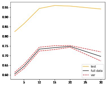
#怎样选取最优的箱子?
#怎样选取最优的箱子?
from sklearn.model_selection import cross_val_score as CVS
import numpy as np
pred,score,var = [], [], []
binsrange = [2,5,10,15,20,30]
for i in binsrange:
    #实例化分箱类
    enc = KBinsDiscretizer(n_bins=i,encode="onehot")
    #转换数据
    X_binned = enc.fit_transform(X)
    line_binned = enc.transform(line)
    #建立模型
    LinearR_ = LinearRegression()
    #全数据集上的交叉验证
    cvresult = CVS(LinearR_,X_binned,y,cv=5) # 交叉验证受到数据量过小的影响,得分不高
    score.append(cvresult.mean())
    var.append(cvresult.var())
    #测试数据集上的打分结果
    pred.append(LinearR_.fit(X_binned,y).score(line_binned,np.sin(line)))
#绘制图像
plt.figure(figsize=(6,5))
plt.plot(binsrange,pred,c="orange",label="test")
plt.plot(binsrange,score,c="k",label="full data")
plt.plot(binsrange,score+np.array(var)*0.5,c="red",linestyle="--",label = "var")
plt.plot(binsrange,score-np.array(var)*0.5,c="red",linestyle="--")
plt.legend()
plt.show()

# 方差越小,模型均值高,模型稳定,泛化能力强
2.2多项式回归PolynomialFeatures
2.2.1多项式对数据的作用
from sklearn.preprocessing import PolynomialFeatures
# 将数据升为,使其在高维空间中成一条直线
import numpy as np
#如果原始数据是一维的
X = np.arange(1,4).reshape(-1,1)
X
array([[1],
       [2],
       [3]])
#二次多项式,参数degree控制多项式的次方
poly = PolynomialFeatures(degree=2)
#接口transform直接调用
X_ = poly.fit_transform(X)
X_
array([[1., 1., 1.],
       [1., 2., 4.],
       [1., 3., 9.]])
X_.shape
(3, 3)
#三次多项式
PolynomialFeatures(degree=3).fit_transform(X)
array([[ 1.,  1.,  1.,  1.],
       [ 1.,  2.,  4.,  8.],
       [ 1.,  3.,  9., 27.]])
#三次多项式,(include_bias=False)不带与截距项相乘的x0
PolynomialFeatures(degree=3,include_bias=False).fit_transform(X)
array([[ 1.,  1.,  1.],
       [ 2.,  4.,  8.],
       [ 3.,  9., 27.]])
#为什么我们会希望不生成与截距相乘的x0呢?
#对于多项式回归来说,我们已经为线性回归准备好了x0,但是线性回归并不知道
xxx = PolynomialFeatures(degree=3).fit_transform(X)
xxx
array([[ 1.,  1.,  1.,  1.],
       [ 1.,  2.,  4.,  8.],
       [ 1.,  3.,  9., 27.]])
xxx.shape
(3, 4)
rnd = np.random.RandomState(42) #设置随机数种子
y = rnd.randn(3)

y
array([ 0.49671415, -0.1382643 , 0.64768854])
#生成了多少个系数?
LinearRegression().fit(xxx,y).coef_
array([ 3.10862447e-15, -3.51045297e-01, -6.06987134e-01, 2.19575463e-01])
#查看截距
# x0的特征的系数应该等于截距,但并没有发生这种情况; 因为线性回归无法判别特征矩阵其中有一列特征是用来成为截距的
# 所以就不多此一举生成一列成为截距(第一列)

# 该模块本身也会自己生成截距
LinearRegression().fit(xxx,y).intercept_
1.2351711202036884
#发现问题了吗?线性回归并没有把多项式生成的x0当作是截距项
#所以我们可以选择:关闭多项式回归中的include_bias
#也可以选择:关闭线性回归中的fit_intercept

#生成了多少个系数?
LinearRegression(fit_intercept=False).fit(xxx,y).coef_

# 生成4个系数,又x0等于1,x0与系数相乘的截距值就是系数值
array([ 1.00596411, 0.06916756, -0.83619415, 0.25777663])
#查看截距
LinearRegression(fit_intercept=False).fit(xxx,y).intercept_
0.0
X = np.arange(6).reshape(3, 2)
X
array([[0, 1],
       [2, 3],
       [4, 5]])
#尝试二次多项式
PolynomialFeatures(degree=2).fit_transform(X)
array([[ 1.,  0.,  1.,  0.,  0.,  1.],
       [ 1.,  2.,  3.,  4.,  6.,  9.],
       [ 1.,  4.,  5., 16., 20., 25.]])
#尝试三次多项式
PolynomialFeatures(degree=3).fit_transform(X)
# 当我们进行多项式转化的时候,多项式会产出最高项为止的所有高低项
array([[  1.,   0.,   1.,   0.,   0.,   1.,   0.,   0.,   0.,   1.],
       [  1.,   2.,   3.,   4.,   6.,   9.,   8.,  12.,  18.,  27.],
       [  1.,   4.,   5.,  16.,  20.,  25.,  64.,  80., 100., 125.]])
PolynomialFeatures(degree=2).fit_transform(X)
array([[ 1.,  0.,  1.,  0.,  0.,  1.],
       [ 1.,  2.,  3.,  4.,  6.,  9.],
       [ 1.,  4.,  5., 16., 20., 25.]])
PolynomialFeatures(degree=2,interaction_only=True).fit_transform(X)
# 比起x1x2类型的二次项,x1x1的共线性更高,可以使用interaction_only=True避免x1次方项带来的高共线性
#对比之下,当interaction_only为True的时候,只生成交互项
array([[ 1.,  0.,  1.,  0.],
       [ 1.,  2.,  3.,  6.],
       [ 1.,  4.,  5., 20.]])
#更高维度的原始特征矩阵
X = np.arange(20).reshape(2, 10)
X
array([[ 0,  1,  2,  3,  4,  5,  6,  7,  8,  9],
       [10, 11, 12, 13, 14, 15, 16, 17, 18, 19]])
PolynomialFeatures(degree=2).fit_transform(X).shape
(2, 66)
PolynomialFeatures(degree=3).fit_transform(X).shape
(2, 286)
X_ = PolynomialFeatures(degree=20).fit_transform(X)

X_.shape
# 维度爆炸上升
# 现实中degree最高就取到7,8;
(2, 30045015)
2.2.2 多项式回归如何处理非线性问题
# 多项式回归如何处理非线性问题
from sklearn.preprocessing import PolynomialFeatures as PF #处理数据
from sklearn.linear_model import LinearRegression
import numpy as np

rnd = np.random.RandomState(42) #设置随机数种子
X = rnd.uniform(-3, 3, size=100)
y = np.sin(X) + rnd.normal(size=len(X)) / 3  #  rnd.normal(size=50) 生成size个随机数

#将X升维,准备好放入sklearn中
X = X.reshape(-1,1)

#创建测试数据,均匀分布在训练集X的取值范围内的一千个点
line = np.linspace(-3, 3, 1000, endpoint=False).reshape(-1, 1)
#原始特征矩阵的拟合结果
LinearR = LinearRegression().fit(X, y)
#对训练数据的拟合
LinearR.score(X,y)
0.5361526059318595
#对测试数据的拟合
LinearR.score(line,np.sin(line))
0.6800102369793313
#多项式拟合,设定高次项
d=5

#进行高次项转换
poly = PF(degree=d)
X_ = poly.fit_transform(X)  #把原始特征矩阵转化为高维特征矩阵
line_ = poly.transform(line) #把测试特征矩阵转化为高维特征矩阵

#训练数据的拟合
LinearR_ = LinearRegression().fit(X_, y)
LinearR_.score(X_,y)
0.8561679370344799
#测试数据的拟合
LinearR_.score(line_,np.sin(line))

# 可以说明多项式回归专门提升模型表现
0.9868904451788011
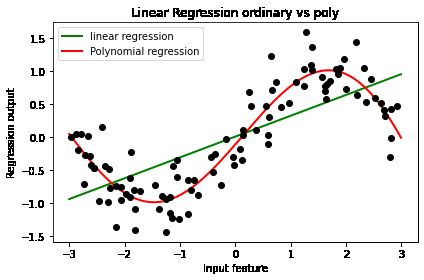
import matplotlib.pyplot as plt

d=5
#和上面展示一致的建模流程
LinearR = LinearRegression().fit(X, y)
X_ = PF(degree=d).fit_transform(X) #把原始特征矩阵转化为高维特征矩阵
LinearR_ = LinearRegression().fit(X_, y)#训练模型
line = np.linspace(-3, 3, 1000, endpoint=False).reshape(-1, 1)#创建测试数据,均匀分布在训练集X的取值范围内的一千个点
line_ = PF(degree=d).fit_transform(line)#把测试特征矩阵转化为高维特征矩阵

#放置画布
fig, ax1 = plt.subplots(1)

#将测试数据带入predict接口,获得模型的拟合效果并进行绘制
ax1.plot(line, LinearR.predict(line), linewidth=2, color='green'
         ,label="linear regression")
ax1.plot(line, LinearR_.predict(line_), linewidth=2, color='red'
         ,label="Polynomial regression")

#将原数据上的拟合绘制在图像上
ax1.plot(X[:, 0], y, 'o', c='k')

#其他图形选项
ax1.legend(loc="best")
ax1.set_ylabel("Regression output")
ax1.set_xlabel("Input feature")
ax1.set_title("Linear Regression ordinary vs poly")
plt.tight_layout()
plt.show()

#来一起鼓掌,感叹多项式回归的神奇

#随后可以试试看较低和较高的次方会发生什么变化
#d=2 欠拟合
#d=20 过拟合
# 可以使用交叉验证找最佳degree
2.2.3 多项式回归的可解释性
# 多项式回归的可解释性
import numpy as np
from sklearn.preprocessing import PolynomialFeatures
from sklearn.linear_model import LinearRegression

X = np.arange(9).reshape(3, 3)
X
array([[0, 1, 2],
       [3, 4, 5],
       [6, 7, 8]])
poly = PolynomialFeatures(degree=5).fit(X)
#重要接口get_feature_names
poly.get_feature_names_out()
array(['1', 'x0', 'x1', 'x2', 'x0^2', 'x0 x1', 'x0 x2', 'x1^2', 'x1 x2',
       'x2^2', 'x0^3', 'x0^2 x1', 'x0^2 x2', 'x0 x1^2', 'x0 x1 x2',
       'x0 x2^2', 'x1^3', 'x1^2 x2', 'x1 x2^2', 'x2^3', 'x0^4', 'x0^3 x1',
       'x0^3 x2', 'x0^2 x1^2', 'x0^2 x1 x2', 'x0^2 x2^2', 'x0 x1^3',
       'x0 x1^2 x2', 'x0 x1 x2^2', 'x0 x2^3', 'x1^4', 'x1^3 x2',
       'x1^2 x2^2', 'x1 x2^3', 'x2^4', 'x0^5', 'x0^4 x1', 'x0^4 x2',
       'x0^3 x1^2', 'x0^3 x1 x2', 'x0^3 x2^2', 'x0^2 x1^3',
       'x0^2 x1^2 x2', 'x0^2 x1 x2^2', 'x0^2 x2^3', 'x0 x1^4',
       'x0 x1^3 x2', 'x0 x1^2 x2^2', 'x0 x1 x2^3', 'x0 x2^4', 'x1^5',
       'x1^4 x2', 'x1^3 x2^2', 'x1^2 x2^3', 'x1 x2^4', 'x2^5'],
      dtype=object)
from sklearn.datasets import fetch_california_housing as fch
import pandas as pd

housevalue = fch()
X = pd.DataFrame(housevalue.data)
y = housevalue.target
housevalue.feature_names
['MedInc',
 'HouseAge',
 'AveRooms',
 'AveBedrms',
 'Population',
 'AveOccup',
 'Latitude',
 'Longitude']
X.columns = ["住户收入中位数","房屋使用年代中位数","平均房间数目"
            ,"平均卧室数目","街区人口","平均入住率","街区的纬度","街区的经度"]
X.head()
| 住户收入中位数 | 房屋使用年代中位数 | 平均房间数目 | 平均卧室数目 | 街区人口 | 平均入住率 | 街区的纬度 | 街区的经度 | |
|---|---|---|---|---|---|---|---|---|
| 0 | 8.3252 | 41.0 | 6.984127 | 1.023810 | 322.0 | 2.555556 | 37.88 | -122.23 |
| 1 | 8.3014 | 21.0 | 6.238137 | 0.971880 | 2401.0 | 2.109842 | 37.86 | -122.22 |
| 2 | 7.2574 | 52.0 | 8.288136 | 1.073446 | 496.0 | 2.802260 | 37.85 | -122.24 |
| 3 | 5.6431 | 52.0 | 5.817352 | 1.073059 | 558.0 | 2.547945 | 37.85 | -122.25 |
| 4 | 3.8462 | 52.0 | 6.281853 | 1.081081 | 565.0 | 2.181467 | 37.85 | -122.25 |
poly = PolynomialFeatures(degree=2).fit(X,y)# 训练模型
poly.get_feature_names_out(X.columns)
array(['1', '住户收入中位数', '房屋使用年代中位数', '平均房间数目', '平均卧室数目', '街区人口', '平均入住率',
       '街区的纬度', '街区的经度', '住户收入中位数^2', '住户收入中位数 房屋使用年代中位数',
       '住户收入中位数 平均房间数目', '住户收入中位数 平均卧室数目', '住户收入中位数 街区人口',
       '住户收入中位数 平均入住率', '住户收入中位数 街区的纬度', '住户收入中位数 街区的经度', '房屋使用年代中位数^2',
       '房屋使用年代中位数 平均房间数目', '房屋使用年代中位数 平均卧室数目', '房屋使用年代中位数 街区人口',
       '房屋使用年代中位数 平均入住率', '房屋使用年代中位数 街区的纬度', '房屋使用年代中位数 街区的经度',
       '平均房间数目^2', '平均房间数目 平均卧室数目', '平均房间数目 街区人口', '平均房间数目 平均入住率',
       '平均房间数目 街区的纬度', '平均房间数目 街区的经度', '平均卧室数目^2', '平均卧室数目 街区人口',
       '平均卧室数目 平均入住率', '平均卧室数目 街区的纬度', '平均卧室数目 街区的经度', '街区人口^2',
       '街区人口 平均入住率', '街区人口 街区的纬度', '街区人口 街区的经度', '平均入住率^2', '平均入住率 街区的纬度',
       '平均入住率 街区的经度', '街区的纬度^2', '街区的纬度 街区的经度', '街区的经度^2'], dtype=object)
X_ = poly.transform(X)
#在这之后,我们依然可以直接建立模型,然后使用线性回归的coef_属性来查看什么特征对标签的影响最大(查看参数w)
reg = LinearRegression().fit(X_,y)
coef = reg.coef_
coef# 每个特征的系数
array([ 5.91956774e-08, -1.12430252e+01, -8.48898547e-01,  6.44105910e+00,
       -3.15913295e+01,  4.06090507e-04,  1.00386233e+00,  8.70568190e+00,
        5.88063272e+00, -3.13081323e-02,  1.85994752e-03,  4.33020546e-02,
       -1.86142285e-01,  5.72831379e-05, -2.59019497e-03, -1.52505718e-01,
       -1.44242941e-01,  2.11725341e-04, -1.26219011e-03,  1.06115056e-02,
        2.81884982e-06, -1.81716946e-03, -1.00690371e-02, -9.99950172e-03,
        7.26947747e-03, -6.89064356e-02, -6.82365771e-05,  2.68878840e-02,
        8.75089896e-02,  8.22890355e-02,  1.60180953e-01,  5.14264167e-04,
       -8.71911437e-02, -4.37043004e-01, -4.04150586e-01,  2.73779399e-09,
        1.91426752e-05,  2.29529768e-05,  1.46567727e-05,  8.71561060e-05,
        2.13344592e-02,  1.62412938e-02,  6.18867358e-02,  1.08107173e-01,
        3.99077350e-02])
[*zip(poly.get_feature_names_out(X.columns),reg.coef_)]# zip合并数据[*]打开惰性对象
[('1', 5.9195677406474074e-08),
 ('住户收入中位数', -11.243025226171353),
 ('房屋使用年代中位数', -0.8488985470451182),
 ('平均房间数目', 6.44105910057414),
 ('平均卧室数目', -31.59132949268304),
 ('街区人口', 0.0004060905068395677),
 ('平均入住率', 1.003862334974344),
 ('街区的纬度', 8.705681895279014),
 ('街区的经度', 5.880632720107474),
 ('住户收入中位数^2', -0.03130813231899294),
 ('住户收入中位数 房屋使用年代中位数', 0.001859947523476963),
 ('住户收入中位数 平均房间数目', 0.04330205461272519),
 ('住户收入中位数 平均卧室数目', -0.1861422845385767),
 ('住户收入中位数 街区人口', 5.7283137863047354e-05),
 ('住户收入中位数 平均入住率', -0.0025901949661491243),
 ('住户收入中位数 街区的纬度', -0.15250571785760378),
 ('住户收入中位数 街区的经度', -0.14424294126438358),
 ('房屋使用年代中位数^2', 0.00021172534135573042),
 ('房屋使用年代中位数 平均房间数目', -0.00126219010601056),
 ('房屋使用年代中位数 平均卧室数目', 0.010611505562750017),
 ('房屋使用年代中位数 街区人口', 2.8188498159276154e-06),
 ('房屋使用年代中位数 平均入住率', -0.0018171694599668443),
 ('房屋使用年代中位数 街区的纬度', -0.010069037145839285),
 ('房屋使用年代中位数 街区的经度', -0.009999501720421652),
 ('平均房间数目^2', 0.007269477468461559),
 ('平均房间数目 平均卧室数目', -0.06890643559321695),
 ('平均房间数目 街区人口', -6.823657707823519e-05),
 ('平均房间数目 平均入住率', 0.02688788402215688),
 ('平均房间数目 街区的纬度', 0.0875089896285016),
 ('平均房间数目 街区的经度', 0.08228903548147115),
 ('平均卧室数目^2', 0.16018095270534952),
 ('平均卧室数目 街区人口', 0.0005142641668794768),
 ('平均卧室数目 平均入住率', -0.0871911436772747),
 ('平均卧室数目 街区的纬度', -0.4370430037140062),
 ('平均卧室数目 街区的经度', -0.40415058610379595),
 ('街区人口^2', 2.7377939915140814e-09),
 ('街区人口 平均入住率', 1.91426752370015e-05),
 ('街区人口 街区的纬度', 2.2952976756807075e-05),
 ('街区人口 街区的经度', 1.4656772717447364e-05),
 ('平均入住率^2', 8.715610601262204e-05),
 ('平均入住率 街区的纬度', 0.021334459218410203),
 ('平均入住率 街区的经度', 0.01624129384963974),
 ('街区的纬度^2', 0.061886735799796935),
 ('街区的纬度 街区的经度', 0.10810717316052239),
 ('街区的经度^2', 0.0399077350075366)]
#放到dataframe中进行排序
coeff = pd.DataFrame([poly.get_feature_names_out(X.columns),reg.coef_.tolist()]).T
coeff.head()
| 0 | 1 | |
|---|---|---|
| 0 | 1 | 0.0 |
| 1 | 住户收入中位数 | -11.243025 |
| 2 | 房屋使用年代中位数 | -0.848899 |
| 3 | 平均房间数目 | 6.441059 |
| 4 | 平均卧室数目 | -31.591329 |
coeff.columns = ["feature","coef"]# 列命名
coeff.sort_values(by="coef")
| feature | coef | |
|---|---|---|
| 4 | 平均卧室数目 | -31.591329 |
| 1 | 住户收入中位数 | -11.243025 |
| 2 | 房屋使用年代中位数 | -0.848899 |
| 33 | 平均卧室数目 街区的纬度 | -0.437043 |
| 34 | 平均卧室数目 街区的经度 | -0.404151 |
| 12 | 住户收入中位数 平均卧室数目 | -0.186142 |
| 15 | 住户收入中位数 街区的纬度 | -0.152506 |
| 16 | 住户收入中位数 街区的经度 | -0.144243 |
| 32 | 平均卧室数目 平均入住率 | -0.087191 |
| 25 | 平均房间数目 平均卧室数目 | -0.068906 |
| 9 | 住户收入中位数^2 | -0.031308 |
| 22 | 房屋使用年代中位数 街区的纬度 | -0.010069 |
| 23 | 房屋使用年代中位数 街区的经度 | -0.01 |
| 14 | 住户收入中位数 平均入住率 | -0.00259 |
| 21 | 房屋使用年代中位数 平均入住率 | -0.001817 |
| 18 | 房屋使用年代中位数 平均房间数目 | -0.001262 |
| 26 | 平均房间数目 街区人口 | -0.000068 |
| 35 | 街区人口^2 | 0.0 |
| 0 | 1 | 0.0 |
| 20 | 房屋使用年代中位数 街区人口 | 0.000003 |
| 38 | 街区人口 街区的经度 | 0.000015 |
| 36 | 街区人口 平均入住率 | 0.000019 |
| 37 | 街区人口 街区的纬度 | 0.000023 |
| 13 | 住户收入中位数 街区人口 | 0.000057 |
| 39 | 平均入住率^2 | 0.000087 |
| 17 | 房屋使用年代中位数^2 | 0.000212 |
| 5 | 街区人口 | 0.000406 |
| 31 | 平均卧室数目 街区人口 | 0.000514 |
| 10 | 住户收入中位数 房屋使用年代中位数 | 0.00186 |
| 24 | 平均房间数目^2 | 0.007269 |
| 19 | 房屋使用年代中位数 平均卧室数目 | 0.010612 |
| 41 | 平均入住率 街区的经度 | 0.016241 |
| 40 | 平均入住率 街区的纬度 | 0.021334 |
| 27 | 平均房间数目 平均入住率 | 0.026888 |
| 44 | 街区的经度^2 | 0.039908 |
| 11 | 住户收入中位数 平均房间数目 | 0.043302 |
| 42 | 街区的纬度^2 | 0.061887 |
| 29 | 平均房间数目 街区的经度 | 0.082289 |
| 28 | 平均房间数目 街区的纬度 | 0.087509 |
| 43 | 街区的纬度 街区的经度 | 0.108107 |
| 30 | 平均卧室数目^2 | 0.160181 |
| 6 | 平均入住率 | 1.003862 |
| 8 | 街区的经度 | 5.880633 |
| 3 | 平均房间数目 | 6.441059 |
| 7 | 街区的纬度 | 8.705682 |
# 不仅数据具有好的解释性,还可以此进行特征组合来创造新特征,实现特征创造
#顺便可以查看一下多项式变化之后,模型的拟合效果如何了
poly = PolynomialFeatures(degree=4).fit(X,y)
X_ = poly.transform(X)
reg = LinearRegression().fit(X,y)
reg.score(X,y)
0.606232685199805
from time import time
time0 = time()
reg_ = LinearRegression().fit(X_,y)
print("R2:{}".format(reg_.score(X_,y)))
print("time:{}".format(time()-time0))
#R^2提升了近15%
R2:0.7454137623736196
time:0.47771406173706055
#假设使用随机森林模型
from sklearn.ensemble import RandomForestRegressor as RFR

time0 = time()
print("R2:{}".format(RFR(n_estimators=100).fit(X,y).score(X,y)))
print("time:{}".format(time()-time0))

# 随机森林效果好,但耗时长;
# 线性模型优势在于速度;
R2:0.9745026675800329
time:9.82259488105774
# 关于多项式回归是线性还是非线性
# 多项式通常被认作非线性模型;

# 狭义线性模型vs广义线性模型
#1.狭义:自变量上不能有高次项
#2.广义:拟合出来的特征之间的系数没有相乘或相除的关系,模型就是线性的
# 多项式变化提升数据维度,增加了过拟合可能,因此多于处理过拟合的线性模型岭回归,lasso共用