Ex3_机器学习_吴恩达课程作业（Python）：多分类和神经网络（Multi-class Classification & Neural Networks）

Ex3_机器学习_吴恩达课程作业（Python）：多分类和神经网络（Multi-class Classification & Neural Networks）

使用说明：

本文章为关于吴恩达老师在Coursera上的机器学习课程的学习笔记。

• 本文第一部分首先介绍课程对应周次的知识回顾以及重点笔记，以及代码实现的库引入。
• 本文第二部分包括代码实现部分中的自定义函数实现细节。
• 本文第三部分即为与课程练习题目相对应的具体代码实现。

0. Pre-condition

This section includes some introductions of libraries.

# This file includes self-created functions used in exercise 3
import numpy as np
import matplotlib.pyplot as plt
import scipy.optimize as opt
from scipy.io import loadmat

00. Self-created Functions

This section includes self-created functions.

• loadData(path)：读取.mat数据

  # Load data from the given file  读取数据
  def loadData(path):
      df = loadmat(path)
      X = df['X']
      y = df['y']
      return X, y
  

• loadWeight(path)：用于前置传播算法，读取神经网络各层的权重数据

  # Load weight data from the given file  读取权重数据
  def loadWeight(path):
      df = loadmat(path)
      return df['Theta1'], df['Theta2']
  

• plotOneImage(X, y)：读取并处理被压缩的灰度图像数据，可视化之

  # Randomly pick a training example and visualize it
  # 随机选取一个训练样本，并且将其可视化
  def plotOneImage(X, y):
      # Randomly pick a number ranging from 0 to the size of given training examples
      index = np.random.randint(0, X.shape[0])
      # Get the data of the random image  获取灰度图像数据
      image_data = X[index, :]
      # Reshape the vector into the gray image matrix  还原被压缩的图像数据向量为20x20数组
      image = image_data.reshape((20, 20))
      # Plot the figure  可视化
      fig, fig_image = plt.subplots(figsize=[4, 4])
      fig_image.matshow(image, cmap='gray_r')
      plt.xticks([])  # 去除图像上的刻度
      plt.yticks([])
      plt.title('Image: ' + format(y[index]))
      # print('This image should be ', format(y[index]))
      plt.show()
  

• plot100Images(X)：读取并处理100条被压缩的灰度图像数据，可视化之

  # Randomly pick 100 training examples and visualize them
  # 随机选取100个训练样本，并且将其可视化
  def plot100Images(X):
      # Randomly pick 100 numbers ranging from 0 to the size of given training examples
      indexes = np.random.choice(np.arange(X.shape[0]), 100)
      # Get the data of random images  获取灰度图像数据
      image_data = X[indexes, :]  # shape: (100, 400)
      # Plot the figure  可视化
      fig, fig_images = plt.subplots(figsize=[8, 8], nrows=10, ncols=10,
                                     sharex=True, sharey=True)
      for row in range(10):
          for col in range(10):
              # Reshape vectors into gray image matrices
              image = image_data[10 * row + col, :].reshape((20, 20))
              fig_images[row, col].matshow(image, cmap='gray_r')
      plt.xticks([])  # 去除图像上的刻度
      plt.yticks([])
      plt.show()
  

• sigmoid(z)：激活函数

  # Sigmoid function  激活函数
  def sigmoid(z):
      return 1 / (1 + np.exp(-z))
  

• logisticRegCost(theta, X, y, l)：计算正规化逻辑回归的损失

  

  

  # Cost function of regularized logistic regression (Vectorized)
  # 向量化计算逻辑回归的损失函数
  # Args: { theta: 训练参数; X: 训练集; y: 标签集; l: 正则化参数lambda }
  def logisticRegCost(theta, X, y, l):
      # Remember not to penalize 'theta_0'
      theta_reg = theta[1:]
      # Compute (tips: both results are a number rather than vector or matrix)
      cost_origin = (-y * np.log(sigmoid(X @ theta))) - (1 - y) * np.log(1 - sigmoid(X @ theta))
      cost_reg = l * (theta_reg @ theta_reg) / (2 * len(X))
      return np.mean(cost_origin) + cost_reg
  

• logisticRegGradient(theta, X, y, l)：计算正规化逻辑回归的梯度

  

  # Gradient of regularized logistic regression (Vectorized)
  # 向量化计算逻辑回归的梯度
  # Args: { theta: 训练参数; X: 训练集; y: 标签集; l: 正则化参数lambda }
  def logisticRegGradient(theta, X, y, l):
      # Remember not to penalize 'theta_0'
      theta_reg = theta[1:]
      # Compute (insert a column of all '0' to avoid penalize on the first column)
      gradient_origin = X.T @ (sigmoid(X @ theta) - y)
      gradient_reg = np.concatenate([np.array([0]), l * theta_reg])
      return (gradient_origin + gradient_reg) / len(X)
  

• oneVsAll(X, y, l, K)：训练一对多分类的分类器，返回参数数组

  # Train on ten classifiers and return final thetas for them
  # 训练十个分类器，并且最终返回一个包含它们最优训练参数的二维数组
  # Args: { X: 训练集; y: 标签集; l: 正则化参数lambda; K: 类别数目 }
  def oneVsAll(X, y, l, K):
      all_theta = np.zeros((K, X.shape[1]))
      for i in range(1, K + 1):
          temp_theta = np.zeros(X.shape[1])
          # Record the true labels
          y_i = np.array([1 if label == i else 0 for label in y])
          # Train
          ret = opt.minimize(fun=logisticRegCost,
                             x0=temp_theta,
                             args=(X, y_i, l),
                             method='TNC',
                             jac=logisticRegGradient,
                             options={'disp': True})
          all_theta[i - 1, :] = ret['x']
      return all_theta
  

• predictOneVsAll(X, all_theta)：用训练得到的多分类器进行预测

  # Predict using the trained multi-class classifiers
  # 用多分类器进行预测，并且返回样本预测值
  # Args: { X: 训练集; all_theta: 训练参数集 }
  def predictOneVsAll(X, all_theta):   
      # Compute class probabilities for each class on every training example
      # 对于每个样本，计算它属于各个类别的可能性
      h = sigmoid(X @ all_theta.T)
      
      # Create an array of indexes with the maximum probability
      # Returns the indices of the maximum values along an axis
      # Since our array was zero-indexed, we need to add one for the true label prediction
      # 获取每一行数据（对每个样本的）的最大值，其对应的下标加一即为该样本最可能属于的类别的下标值
      # index_max数组包含对所有训练样本的预测值（所属类别），即此处为5000行
      # 由于数组操作时下标从零开始，此处我们需要为其加一
      index_max = np.argmax(h, axis=1) + 1
      
      return index_max
  

1. Multi-class Classification

For this exercise, you will use logistic regression and neural networks to recognize handwritten digits (from 0 to 9).

Automated handwritten digit recognition is widely used today - from recognizing zip codes (postal codes) on mail envelopes to recognizing amounts written on bank checks.

This exercise will show you how the methods you’ve learned can be used for this classifification task.

• 调用的相关函数在文章头部"Self-created functions"中详细描述。

我们将扩展我们在ex_2中写的logistic回归的实现，并将其应用于一对多的分类。

1.1 Dataset

首先，加载数据集。这里的数据为.mat的格式，所以要使用scipy.io的loadmat函数。

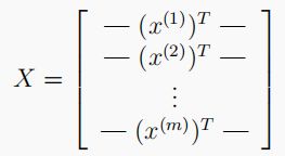
• 数据集中有5000个训练样本，每个样本是 $20x20$​​​ 像素的数字的灰度图像。每个像素代表一个浮点数，表示该位置的灰度强度。$20\times 20$​​ 的像素网格被展开成一个 $400$​ ​维的向量。在我们的数据矩阵 $X$​​ 中，每一个样本都变成了一行，这给了我们一个 $5000\times 400$​​ 矩阵 $X$​​​ ，每一行都是一个手写数字图像的训练样本。
• 数据集的第二部分是一个$5000$维的向量 $y$ ，它包含训练集的标签。

# 1. Multi-class classification 多分类问题

# 1.1 Dataset  数据集处理
path = '../data/ex3data1.mat'
raw_X, raw_y = func.loadData(path)
X = np.insert(raw_X, 0, 1, axis=1)
y = raw_y.flatten()
print(np.unique(raw_y))  # 查看标签种类 [1, 2, 3, 4, 5, 6, 7, 8, 9, 10]

1.2 Visualization

这部分代码随机从数据集$X$​中选择$100$​​​​行并传递这些行到displayData函数。该函数将每行数据映射为 $20x20$​​ 像素的灰度图像并且最终将图像集中显示。期望输出图像为如下：

# 1.2 Visualization  可视化
func.plotOneImage(raw_X, raw_y)
func.plot100Images(raw_X)

1.3 Vectorize Logistic Regression

此时，将使用多个one-vs-all logistic model来构建一个多分类器。因为有10个分类，需要训练10个独立的logistic regression classifiers。为了使训练更有效，需要确保您的代码是良好的向量化。第一个任务是将我们的逻辑回归实现修改为完全向量化（即没有for循环）。这是因为向量化代码除了简洁外，还能够利用线性代数优化，并且通常比迭代代码快得多。

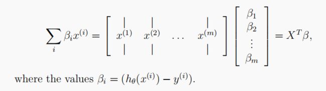
# 1.3 Vectorize Logistic Regression  向量化逻辑回归
res_cost = func.logisticRegCost(all_theta, X, y, l=1)  # all_theta在之后的代码中定义
res_gradient = func.logisticRegGradient(all_theta, X, y, l=1)
print(res_cost)
print(res_gradient)

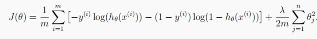
1.3.1 Cost function

正则化的logistic回归的代价函数是：

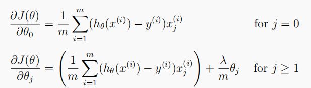
1.3.2 Gradient

正则化logistic回归代价函数的梯度下降法如下表示，因为不惩罚 $thet{a}_0$​ ，所以分为两种情况：

1.4 One-vs-all Classification

在本部分，将通过训练多个正则化逻辑回归分类器来实现“一对多分类”，每个类别对应数据集 $K$ 类中的一个。

对于这个任务，我们有10个可能的类，并且由于logistic回归只能一次在2个类之间进行分类，每个分类器在“属于类别 i”和“不属于类别i”之间决定。 我们将把分类器训练包含在一个函数中，该函数计算10个分类器中的每个分类器的最终权重，并将权重返回shape为 $(k,(n+1))$​ 的数组，其中 $n$​ 是参数数量。

# 1.4 One-vs-all Classification 一对多分类
all_theta = func.oneVsAll(X, y, l=1, K=10)
predictions = func.predictOneVsAll(X, all_theta)
accuracy = np.mean(predictions == y)
print('accuracy = ' + format(accuracy * 100) + '%')

这里的 $h$ 共 $5000$ 行，$10$ 列，每行代表一个样本，每列是预测对应数字的概率。我们取概率最大对应的下标加 $1$ 就是我们分类器最终预测出来的类别。此外，最终返回的 $h\_argmax$ 是一个数组，包含 $5000$ 个样本对应的预测值。

2. Neural Networks

This section includes some details of exploring “neural networks”.

• 调用的相关函数在文章头部"Self-created functions"中详细描述。

第一章节使用多类logistic回归，然而logistic回归不能形成更复杂的假设，因为它只是一个线性分类器。

接下来我们用neural network (神经网络)来尝试下，神经网络可以实现非常复杂的非线性模型。我们将利用已经训练好了的权重进行预测。

# 2. Neural Networks  神经网络
path = '../data/ex3weights.mat'
theta1, theta2 = func.loadWeight(path)
print(theta1.shape)
print(theta2.shape)

2.1 Model Representation

训练样本X从1开始逐渐增加，训练出不同的参数向量θ。接着通过交叉验证样本Xval计算验证误差。

1. 使用训练集的子集来训练模型，得到不同的θ。
2. 通过θ计算训练代价和交叉验证代价，切记此时不要使用正则化，将$\lambda =0$。
3. 计算交叉验证代价时记得整个交叉验证集来计算，无需分为子集。

# 2.1 Model Representation  模型表示
X, y = func.loadData('ex3data1.mat')
X = np.insert(X, 0, values=np.ones(X.shape[0]), axis=1)
y = y.flatten()

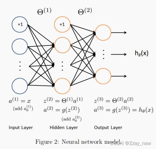
2.2 Feed Forward Propagation and Prediction

# 2.2 Feedforward propagation and prediction  前向传播算法
# Every hidden layer should be inserted with a bias unit  记得插入偏置单元

# Input layer 输入层
a1 = X

# Hidden layer 隐藏层
z2 = a1 @ theta1.T
z2 = np.insert(z2, 0, 1, axis=1)
a2 = func.sigmoid(z2)

# Output layer 输出层
z3 = a2 @ theta2.T
a3 = func.sigmoid(z3)

# Make predictions 做出预测
y_predictions = np.argmax(a3, axis=1) + 1
accuracy = np.mean(y_predictions == y)
print('accuracy = ' + format(accuracy * 100) + '%')