机器学习之支持向量机实例,线性核函数 多项式核函数 RBF高斯核函数 sigmoid核函数
文章目录
- 支持向量机实例
-
- 1.线性核函数
- 2.多项式核函数
- 3.RBF高斯核函数
- 4.sigmoid核函数
- 代码:
- 结果:
支持向量机实例
1.线性核函数
def test_SVC_linear():
    '''
    测试 SVC 的用法。这里使用的是最简单的线性核
    :param data:  可变参数。它是一个元组,这里要求其元素依次为训练样本集、测试样本集、训练样本的标记、测试样本的标记
    :return: None
    '''
    iris = datasets.load_iris()
    X_train, X_test, y_train, y_test=train_test_split(iris.data, iris.target, test_size=0.25,
		random_state=0,stratify=iris.target)
    cls=SVC(kernel='linear')
    cls.fit(X_train,y_train)
    print('Coefficients:%s, intercept %s'%(cls.coef_,cls.intercept_))
    print('Score: %.2f' % cls.score(X_test, y_test))
2.多项式核函数
def test_SVC_poly():
    '''
    测试多项式核的 SVC 的预测性能随 degree、gamma、coef0 的影响.
    :param data:  可变参数。它是一个元组,这里要求其元素依次为训练样本集、测试样本集、训练样本的标记、测试样本的标记
    :return: None
    '''
    iris = datasets.load_iris()
    X_train, X_test, y_train, y_test = train_test_split(iris.data, iris.target, test_size=0.25,
                                                        random_state=0, stratify=iris.target)
    fig=plt.figure()
    ### 测试 degree ####
    degrees=range(1,20)
    train_scores=[]
    test_scores=[]
    for degree in degrees:
        cls=SVC(kernel='poly',degree=degree,gamma='auto')
        cls.fit(X_train,y_train)
        train_scores.append(cls.score(X_train,y_train))
        test_scores.append(cls.score(X_test, y_test))
    ax=fig.add_subplot(1,3,1) # 一行三列
    ax.plot(degrees,train_scores,label="Training score ",marker='+' )
    ax.plot(degrees,test_scores,label= " Testing  score ",marker='o' )
    ax.set_title( "SVC_poly_degree ")
    ax.set_xlabel("p")
    ax.set_ylabel("score")
    ax.set_ylim(0,1.05)
    ax.legend(loc="best",framealpha=0.5)

    ### 测试 gamma ,此时 degree 固定为 3####
    gammas=range(1,20)
    train_scores=[]
    test_scores=[]
    for gamma in gammas:
        cls=SVC(kernel='poly',gamma=gamma,degree=3)
        cls.fit(X_train,y_train)
        train_scores.append(cls.score(X_train,y_train))
        test_scores.append(cls.score(X_test, y_test))
    ax=fig.add_subplot(1,3,2)
    ax.plot(gammas,train_scores,label="Training score ",marker='+' )
    ax.plot(gammas,test_scores,label= " Testing  score ",marker='o' )
    ax.set_title( "SVC_poly_gamma ")
    ax.set_xlabel(r"$\gamma$")
    ax.set_ylabel("score")
    ax.set_ylim(0,1.05)
    ax.legend(loc="best",framealpha=0.5)

    ### 测试 r ,此时 gamma固定为10 , degree 固定为 3######
    rs=range(0,20)
    train_scores=[]
    test_scores=[]
    for r in rs:
        cls=SVC(kernel='poly',gamma=10,degree=3,coef0=r)
        cls.fit(X_train,y_train)
        train_scores.append(cls.score(X_train,y_train))
        test_scores.append(cls.score(X_test, y_test))
    ax=fig.add_subplot(1,3,3)
    ax.plot(rs,train_scores,label="Training score ",marker='+' )
    ax.plot(rs,test_scores,label= " Testing  score ",marker='o' )
    ax.set_title( "SVC_poly_r ")
    ax.set_xlabel(r"r")
    ax.set_ylabel("score")
    ax.set_ylim(0,1.05)
    ax.legend(loc="best",framealpha=0.5)
    plt.show()
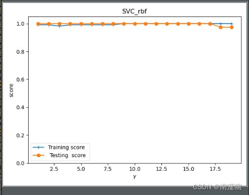
3.RBF高斯核函数
ef test_SVC_rbf():
    '''
    测试 高斯核的 SVC 的预测性能随 gamma 参数的影响
    :param data:  可变参数。它是一个元组,这里要求其元素依次为训练样本集、测试样本集、训练样本的标记、测试样本的标记
    :return: None
    '''
    iris = datasets.load_iris()
    X_train, X_test, y_train, y_test=train_test_split(iris.data, iris.target, test_size=0.25,
		random_state=0,stratify=iris.target)
    gammas=range(1,20)
    train_scores=[]
    test_scores=[]
    for gamma in gammas:
        cls=SVC(kernel='rbf',gamma=gamma)
        cls.fit(X_train,y_train)
        train_scores.append(cls.score(X_train,y_train))
        test_scores.append(cls.score(X_test, y_test))

    fig=plt.figure()
    ax=fig.add_subplot(1,1,1)
    ax.plot(gammas,train_scores,label="Training score ",marker='+' )
    ax.plot(gammas,test_scores,label= " Testing  score ",marker='o' )
    ax.set_title( "SVC_rbf")
    ax.set_xlabel(r"$\gamma$")
    ax.set_ylabel("score")
    ax.set_ylim(0,1.05)
    ax.legend(loc="best",framealpha=0.5)
    plt.show()
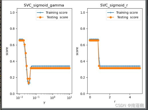
4.sigmoid核函数
def test_SVC_sigmoid():
    '''
    测试 sigmoid 核的 SVC 的预测性能随 gamma、coef0 的影响.
    :param data:  可变参数。它是一个元组,这里要求其元素依次为训练样本集、测试样本集、训练样本的标记、测试样本的标记
    :return: None
    '''
    iris = datasets.load_iris()
    X_train, X_test, y_train, y_test=train_test_split(iris.data, iris.target, test_size=0.25,
		random_state=0,stratify=iris.target)
    fig=plt.figure()

    ### 测试 gamma ,固定 coef0 为 0 ####
    gammas=np.logspace(-2,1)
    train_scores=[]
    test_scores=[]

    for gamma in gammas:
        cls=SVC(kernel='sigmoid',gamma=gamma,coef0=0)
        cls.fit(X_train,y_train)
        train_scores.append(cls.score(X_train,y_train))
        test_scores.append(cls.score(X_test, y_test))
    ax=fig.add_subplot(1,2,1)
    ax.plot(gammas,train_scores,label="Training score ",marker='+' )
    ax.plot(gammas,test_scores,label= " Testing  score ",marker='o' )
    ax.set_title( "SVC_sigmoid_gamma ")
    ax.set_xscale("log")
    ax.set_xlabel(r"$\gamma$")
    ax.set_ylabel("score")
    ax.set_ylim(0,1.05)
    ax.legend(loc="best",framealpha=0.5)

    ### 测试 r,固定 gamma 为 0.01 ######
    rs=np.linspace(0,5)
    train_scores=[]
    test_scores=[]

    for r in rs:
        cls=SVC(kernel='sigmoid',coef0=r,gamma=0.01)
        cls.fit(X_train,y_train)
        train_scores.append(cls.score(X_train,y_train))
        test_scores.append(cls.score(X_test, y_test))
    ax=fig.add_subplot(1,2,2)
    ax.plot(rs,train_scores,label="Training score ",marker='+' )
    ax.plot(rs,test_scores,label= " Testing  score ",marker='o' )
    ax.set_title( "SVC_sigmoid_r ")
    ax.set_xlabel(r"r")
    ax.set_ylabel("score")
    ax.set_ylim(0,1.05)
    ax.legend(loc="best",framealpha=0.5)
    plt.show()
代码:
import numpy as np
from sklearn import datasets
from sklearn.model_selection import train_test_split
from sklearn.svm import SVC
import matplotlib.pyplot as plt


def test_SVC_linear():
    '''
    测试 SVC 的用法。这里使用的是最简单的线性核
    :param data:  可变参数。它是一个元组,这里要求其元素依次为训练样本集、测试样本集、训练样本的标记、测试样本的标记
    :return: None
    '''
    iris = datasets.load_iris()
    X_train, X_test, y_train, y_test=train_test_split(iris.data, iris.target, test_size=0.25,
		random_state=0,stratify=iris.target)
    cls=SVC(kernel='linear')
    cls.fit(X_train,y_train)
    print('Coefficients:%s, intercept %s'%(cls.coef_,cls.intercept_))
    print('Score: %.2f' % cls.score(X_test, y_test))

def test_SVC_poly():
    '''
    测试多项式核的 SVC 的预测性能随 degree、gamma、coef0 的影响.
    :param data:  可变参数。它是一个元组,这里要求其元素依次为训练样本集、测试样本集、训练样本的标记、测试样本的标记
    :return: None
    '''
    iris = datasets.load_iris()
    X_train, X_test, y_train, y_test = train_test_split(iris.data, iris.target, test_size=0.25,
                                                        random_state=0, stratify=iris.target)
    fig=plt.figure()
    ### 测试 degree ####
    degrees=range(1,20)
    train_scores=[]
    test_scores=[]
    for degree in degrees:
        cls=SVC(kernel='poly',degree=degree,gamma='auto')
        cls.fit(X_train,y_train)
        train_scores.append(cls.score(X_train,y_train))
        test_scores.append(cls.score(X_test, y_test))
    ax=fig.add_subplot(1,3,1) # 一行三列
    ax.plot(degrees,train_scores,label="Training score ",marker='+' )
    ax.plot(degrees,test_scores,label= " Testing  score ",marker='o' )
    ax.set_title( "SVC_poly_degree ")
    ax.set_xlabel("p")
    ax.set_ylabel("score")
    ax.set_ylim(0,1.05)
    ax.legend(loc="best",framealpha=0.5)

    ### 测试 gamma ,此时 degree 固定为 3####
    gammas=range(1,20)
    train_scores=[]
    test_scores=[]
    for gamma in gammas:
        cls=SVC(kernel='poly',gamma=gamma,degree=3)
        cls.fit(X_train,y_train)
        train_scores.append(cls.score(X_train,y_train))
        test_scores.append(cls.score(X_test, y_test))
    ax=fig.add_subplot(1,3,2)
    ax.plot(gammas,train_scores,label="Training score ",marker='+' )
    ax.plot(gammas,test_scores,label= " Testing  score ",marker='o' )
    ax.set_title( "SVC_poly_gamma ")
    ax.set_xlabel(r"$\gamma$")
    ax.set_ylabel("score")
    ax.set_ylim(0,1.05)
    ax.legend(loc="best",framealpha=0.5)

    ### 测试 r ,此时 gamma固定为10 , degree 固定为 3######
    rs=range(0,20)
    train_scores=[]
    test_scores=[]
    for r in rs:
        cls=SVC(kernel='poly',gamma=10,degree=3,coef0=r)
        cls.fit(X_train,y_train)
        train_scores.append(cls.score(X_train,y_train))
        test_scores.append(cls.score(X_test, y_test))
    ax=fig.add_subplot(1,3,3)
    ax.plot(rs,train_scores,label="Training score ",marker='+' )
    ax.plot(rs,test_scores,label= " Testing  score ",marker='o' )
    ax.set_title( "SVC_poly_r ")
    ax.set_xlabel(r"r")
    ax.set_ylabel("score")
    ax.set_ylim(0,1.05)
    ax.legend(loc="best",framealpha=0.5)
    plt.show()

def test_SVC_rbf():
    '''
    测试 高斯核的 SVC 的预测性能随 gamma 参数的影响
    :param data:  可变参数。它是一个元组,这里要求其元素依次为训练样本集、测试样本集、训练样本的标记、测试样本的标记
    :return: None
    '''
    iris = datasets.load_iris()
    X_train, X_test, y_train, y_test=train_test_split(iris.data, iris.target, test_size=0.25,
		random_state=0,stratify=iris.target)
    gammas=range(1,20)
    train_scores=[]
    test_scores=[]
    for gamma in gammas:
        cls=SVC(kernel='rbf',gamma=gamma)
        cls.fit(X_train,y_train)
        train_scores.append(cls.score(X_train,y_train))
        test_scores.append(cls.score(X_test, y_test))

    fig=plt.figure()
    ax=fig.add_subplot(1,1,1)
    ax.plot(gammas,train_scores,label="Training score ",marker='+' )
    ax.plot(gammas,test_scores,label= " Testing  score ",marker='o' )
    ax.set_title( "SVC_rbf")
    ax.set_xlabel(r"$\gamma$")
    ax.set_ylabel("score")
    ax.set_ylim(0,1.05)
    ax.legend(loc="best",framealpha=0.5)
    plt.show()

def test_SVC_sigmoid():
    '''
    测试 sigmoid 核的 SVC 的预测性能随 gamma、coef0 的影响.
    :param data:  可变参数。它是一个元组,这里要求其元素依次为训练样本集、测试样本集、训练样本的标记、测试样本的标记
    :return: None
    '''
    iris = datasets.load_iris()
    X_train, X_test, y_train, y_test=train_test_split(iris.data, iris.target, test_size=0.25,
		random_state=0,stratify=iris.target)
    fig=plt.figure()

    ### 测试 gamma ,固定 coef0 为 0 ####
    gammas=np.logspace(-2,1)
    train_scores=[]
    test_scores=[]

    for gamma in gammas:
        cls=SVC(kernel='sigmoid',gamma=gamma,coef0=0)
        cls.fit(X_train,y_train)
        train_scores.append(cls.score(X_train,y_train))
        test_scores.append(cls.score(X_test, y_test))
    ax=fig.add_subplot(1,2,1)
    ax.plot(gammas,train_scores,label="Training score ",marker='+' )
    ax.plot(gammas,test_scores,label= " Testing  score ",marker='o' )
    ax.set_title( "SVC_sigmoid_gamma ")
    ax.set_xscale("log")
    ax.set_xlabel(r"$\gamma$")
    ax.set_ylabel("score")
    ax.set_ylim(0,1.05)
    ax.legend(loc="best",framealpha=0.5)

    ### 测试 r,固定 gamma 为 0.01 ######
    rs=np.linspace(0,5)
    train_scores=[]
    test_scores=[]

    for r in rs:
        cls=SVC(kernel='sigmoid',coef0=r,gamma=0.01)
        cls.fit(X_train,y_train)
        train_scores.append(cls.score(X_train,y_train))
        test_scores.append(cls.score(X_test, y_test))
    ax=fig.add_subplot(1,2,2)
    ax.plot(rs,train_scores,label="Training score ",marker='+' )
    ax.plot(rs,test_scores,label= " Testing  score ",marker='o' )
    ax.set_title( "SVC_sigmoid_r ")
    ax.set_xlabel(r"r")
    ax.set_ylabel("score")
    ax.set_ylim(0,1.05)
    ax.legend(loc="best",framealpha=0.5)
    plt.show()

if __name__=="__main__":
    test_SVC_linear()
    test_SVC_poly()
    test_SVC_rbf()
    test_SVC_sigmoid()
结果:
线性核函数

多项式核函数

RBF高斯核函数
sigmoid核函数