d3_10_Introduction to Artificial Neural Network w Keras1_HuberLoss_astype_dtype_DNN_MLP_G.gv.pdf_EMA
![]() Birds inspired us to fly, burdock plants inspired Velcro, and nature has inspired countless more inventions. It seems only logical, then, to look at the brain's architecture for inspiration on how to build an intelligent machine. This is the logic that sparked artificial neural networks (ANNs): an ANN is a Machine Learning model inspired by the networks of biological neurons found in our brains. However, although planes were inspired by birds, they don't have to flap their wings. Similarly, ANNs have gradually become quite different from their biological cousins. Some researchers even argue that we should drop the biological analogy altogether (e.g., by saying “units” rather than “neurons”), lest we restrict our creativity to biologically plausible systems.
Birds inspired us to fly, burdock plants inspired Velcro, and nature has inspired countless more inventions. It seems only logical, then, to look at the brain's architecture for inspiration on how to build an intelligent machine. This is the logic that sparked artificial neural networks (ANNs): an ANN is a Machine Learning model inspired by the networks of biological neurons found in our brains. However, although planes were inspired by birds, they don't have to flap their wings. Similarly, ANNs have gradually become quite different from their biological cousins. Some researchers even argue that we should drop the biological analogy altogether (e.g., by saying “units” rather than “neurons”), lest we restrict our creativity to biologically plausible systems.
ANNs are at the very core of Deep Learning. They are versatile多用途的, powerful, and scalable, making them ideal to tackle large and highly complex Machine Learning tasks such as classifying billions of images (e.g., Google Images), powering speech recognition services (e.g., Apple’s Siri), recommending the best videos to watch to hundreds of millions of users every day (e.g., YouTube), or learning to beat the world champion at the game of Go (DeepMind's AlphaGo).
The first part of this chapter introduces artificial neural networks, starting with a quick tour of the very first ANN architectures and leading up to Multilayer Perceptrons (MLPs), which are heavily used today (other architectures will be explored in the next chapters). In the second part, we will look at how to implement neural networks using the popular Keras API. This is a beautifully designed and simple high-level API for building, training, evaluating, and running neural networks. But don't be fooled by its simplicity: it is expressive and flexible enough to let you build a wide variety of neural network architectures. In fact, it will probably be sufficient for most of your use cases. And should you ever need extra flexibility, you can always write custom Keras components using its lower-level API, as we will see in Chapter 12.
But first, let’s go back in time to see how artificial neural networks came to be!
From Biological to Artificial Neurons
Surprisingly, ANNs have been around for quite a while: they were first introduced back in 1943 by the neurophysiologist Warren McCulloch and the mathematician Walter Pitts. In their landmark paper2 “A Logical Calculus of Ideas Immanent内在的 in Nervous Activity,” McCulloch and Pitts presented a simplified computational model of how biological neurons might work together in animal brains to perform complex computations using propositional命题 logic. This was the first artificial neural network architecture. Since then many other architectures have been invented, as we will see.
The early successes of ANNs led to the widespread belief that we would soon be conversing交流 with truly intelligent machines. When it became clear in the 1960s that this promise would go unfulfilled (at least for quite a while), funding flew elsewhere, and ANNs entered a long winter. In the early 1980s, new architectures were invented and better training techniques were developed, sparking a revival复兴 of interest in connectionism (the study of neural networks). But progress was slow, and by the 1990s other powerful Machine Learning techniques were invented, such as Support Vector Machines (see https://blog.csdn.net/Linli522362242/article/details/104151351). These techniques seemed to offer better results and stronger theoretical foundations than ANNs, so once again the study of neural networks was put on hold搁置.
We are now witnessing yet another wave of interest in ANNs. Will this wave die out like the previous ones did? Well, here are a few good reasons to believe that this time is different and that the renewed interest in ANNs will have a much more profound深刻 impact on our lives:
- There is now a huge quantity of data available to train neural networks, and ANNs frequently outperform other ML techniques on very large and complex problems.
- The tremendous increase in computing power since the 1990s now makes it possible to train large neural networks in a reasonable amount of time. This is in part due to Moore's摩尔 law (the number of components in integrated circuits has doubled about every 2 years over the last 50 years), but also thanks to the gaming industry, which has stimulated刺激 the production of powerful GPU cards by the millions. Moreover, cloud platforms have made this power accessible to everyone.
- The training algorithms have been improved. To be fair they are only slightly different from the ones used in the 1990s, but these relatively small tweaks have had a huge positive impact.
- Some theoretical limitations of ANNs have turned out to be benign良性的 in practice. For example, many people thought that ANN training algorithms were doomed because they were likely to get stuck in local optima, but it turns out that this is rather rare in practice (and when it is the case, they are usually fairly close to the global optimum).
- ANNs seem to have entered a virtuous有道德 circle of funding and progress. Amazing products based on ANNs regularly make the headline news, which pulls more and more attention and funding toward them, resulting in more and more progress and even more amazing products.
Biological Neurons
Before we discuss artificial neurons, let's take a quick look at a biological neuron (represented in Figure 10-1). It is an unusual-looking cell mostly found in animal brains. It's composed of a cell body containing the nucleus and most of the cell's complex components, many branching extensions called dendrites树突, plus one very long extension called the axon轴突. The axon's length may be just a few times longer than the cell body, or up to tens of thousands of times longer. Near its extremity端点 the axon splits off into many branches called telodendria终树突, and at the tip of these branches are minuscule微小的 structures called synaptic突触的 terminals (or simply synapses)突触, which are connected to the dendrites or cell bodies of other neurons. Biological neurons produce short electrical impulses called action potentials动作电位 (APs, or just signals) which travel along the axons and make the synapses release chemical signals called neurotransmitters神经递质. When a neuron receives a sufficient amount of these neurotransmitters within a few milliseconds, it fires its own electrical impulses (actually, it depends on the neurotransmitters, as some of them inhibit the neuron from firing).
Figure 10-1. Biological neuron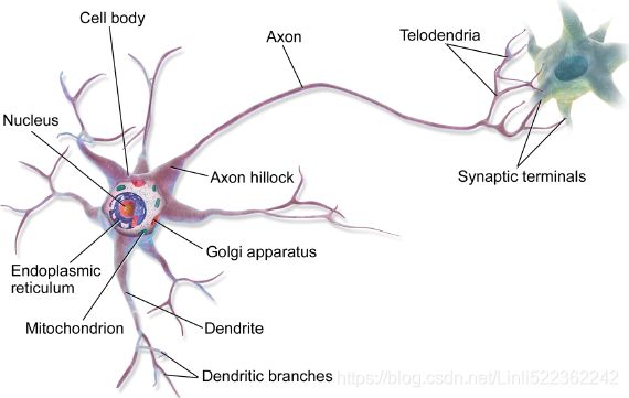
Thus, individual biological neurons seem to behave in a rather simple way, but they are organized in a vast network of billions, with each neuron typically connected to thousands of other neurons. Highly complex computations can be performed by a network of fairly simple neurons, much like a complex anthill垤 can emerge from the combined efforts of simple ants. The architecture of biological neural networks (BNNs) is still the subject of active research, but some parts of the brain have been mapped, and it seems that neurons are often organized in consecutive layers, especially in the cerebral大脑神经 cortex 皮质 (i.e., the outer layer of your brain), as shown in Figure 10-2.
Figure 10-2. Multiple layers in a biological neural network (human cortex)
Logical Computations with Neurons
McCulloch and Pitts proposed a very simple model of the biological neuron, which later became known as an artificial neuron: it has one or more binary (on/off) inputs and one binary output. The artificial neuron activates its output when more than a certain number of its inputs are active. In their paper, they showed that even with such a simplified model it is possible to build a network of artificial neurons that computes any logical proposition you want. To see how such a network works, let's build a few ANNs that perform various logical computations (see Figure 10-3), assuming that a neuron is activated when at least two of its inputs are active.
Figure 10-3. ANNs performing simple logical computations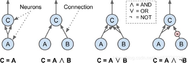
Let's see what these networks do:
- The first network on the left is the identity function: if neuron A is activated, then neuron C gets activated as well (since it receives two input signals from neuron A); but if neuron A is off, then neuron C is off as well.
- The second network performs a logical AND: neuron C is activated only when both neurons A and B are activated (a single input signal is not enough to activate neuron C).
- The third network performs a logical OR: neuron C gets activated if either neuron A or neuron B is activated (or both).
- Finally, if we suppose that an input connection can inhibit抑制 the neuron's activity (which is the case with biological neurons), then the fourth network computes a slightly more complex logical proposition: neuron C is activated only if neuron A is active and neuron B is off. If neuron A is active all the time, then you get a logical NOT: neuron C is active when neuron B is off, and vice versa.
You can imagine how these networks can be combined to compute complex logical expressions (see the exercises at the end of the chapter for an example).
The Perceptron
The Perceptron is one of the simplest ANN architectures, invented in 1957 by Frank Rosenblatt. It is based on a slightly different artificial neuron (see Figure 10-4) called a threshold logic unit (TLU), or sometimes a linear threshold unit (LTU). The inputs and output are numbers (instead of binary on/off values), and each input connection is associated with a weight. The TLU computes a weighted sum of its inputs (![]() ), then applies a step function to that sum and outputs the result:
), then applies a step function to that sum and outputs the result: ![]() , where
, where ![]() .
.
Figure 10-4. Threshold logic unit: an artificial neuron which computes a weighted sum of its inputs then applies a step function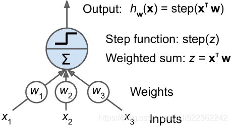
Equation 10-1. Common step functions used in Perceptrons (assuming threshold =0)
A single LTU can be used for simple linear binary classification. It computes a linear combination of the inputs and if the result exceeds a threshold, it outputs the positive class or else outputs the negative class (just like a Logistic Regression classifier or a linear SVM). For example, you could use a single LTU to classify iris flowers based on the petal length and width (also adding an extra bias feature x0 = 1, just like we did in previous chapters). Training an LTU(OR TLU) means finding the right values for ![]() (the training algorithm is discussed shortly).
(the training algorithm is discussed shortly).
A Perceptron is simply composed of a single layer of TLUs, with each TLU connected to all the inputs. When all the neurons in a layer are connected to every neuron in the previous layer (i.e., its input neurons), the layer is called a fully connected layer, or a dense layer. The inputs of the Perceptron are fed to special passthrough neurons called input neurons: they output whatever input they are fed. All the input neurons form the input layer. Moreover, an extra bias feature is generally added (![]() = 1): it is typically represented using a special type of neuron called a bias neuron, which outputs 1 all the time. A Perceptron with two inputs and three outputs is represented in Figure 10-5. This Perceptron can classify instances simultaneously into three different binary classes, which makes it a multioutput classifier.
= 1): it is typically represented using a special type of neuron called a bias neuron, which outputs 1 all the time. A Perceptron with two inputs and three outputs is represented in Figure 10-5. This Perceptron can classify instances simultaneously into three different binary classes, which makes it a multioutput classifier.
Figure 10-5. Architecture of a Perceptron with two input neurons, one bias neuron, and three output neurons
Thanks to the magic of linear algebra, Equation 10-2 makes it possible to efficiently compute the outputs of a layer of artificial neurons for several instances at once.
Equation 10-2. Computing the outputs of a fully connected layer![]()
In this equation:
- As always, X represents the matrix of input features. It has one row per instance and one column per feature.
- The weight matrix W contains all the connection weights except for the ones from the bias neuron. It has one row per input neuron and one column per artificial neuron in the layer.
- The bias vector b contains all the connection weights between the bias neuron and the artificial neurons. It has one bias term per artificial neuron.
- The function ϕ is called the activation function: when the artificial neurons are TLUs, it is a step function (but we will discuss other activation functions shortly).
So, how is a Perceptron trained? The Perceptron training algorithm proposed by Rosenblatt was largely inspired by Hebb's rule. In his 1949 book The Organization of Behavior (Wiley), Donald Hebb suggested that when a biological neuron triggers another neuron often, the connection between these two neurons grows stronger. Siegrid Löwel later summarized Hebb's idea in the catchy phrase, “Cells that fire together, wire together"; that is, the connection weight between two neurons tends to increase when they fire simultaneously. This rule later became known as Hebb's rule
(or Hebbian learning). Perceptrons are trained using a variant of this rule that takes into account the error made by the network when it makes a prediction; the Perceptron learning rule reinforces connections that help reduce the error. More
specifically, the Perceptron is fed one training instance at a time, and for each instance it makes its predictions. For every output neuron that produced a wrong prediction, it reinforces the connection weights from the inputs that would have contributed to the correct prediction. The rule is shown in Equation 10-3.
Equation 10-3. Perceptron learning rule (weight update)![]()
In this equation:
 is the connection weight between the
  input neuron and the
  output neuron.
 is the
  input value of the current training instance.
 is the output of the
  output neuron for the current training instance. # the predicted class label
 is the target output of the
  output neuron for the current training instance. # the true class label
- η is the learning rate.
 https://blog.csdn.net/Linli522362242/article/details/96429442
The decision boundary of each output neuron is linear, so Perceptrons are incapable of learning complex patterns (just like Logistic Regression classifiers). However, if the training instances are linearly separable, Rosenblatt demonstrated that this algorithm would converge to a solution. This is called the Perceptron convergence theorem.
Scikit-Learn provides a Perceptron class that implements a single-TLU network. It can be used pretty much as you would expect—for example, on the iris dataset (introduced in https://blog.csdn.net/Linli522362242/article/details/104097191):
import numpy as np
from sklearn.datasets import load_iris
from sklearn.linear_model import Perceptron

iris = load_iris()
iris![]()
X = iris.data[ :, (2,3) ] # petal length, petal width
y = ( iris.target == 0 ).astype( np.int ) # Iris Setosa

per_clf = Perceptron(max_iter = 1000, tol=1e-3, random_state=42)
per_clf.fit(X,y)

y_pred = per_clf.predict([[ 2,0.5 ]]) # [[petal length, petal width]] # must 2D array
y_pred![]()
# Separating hyperplane
# w0*x0 + w1*x1 + b =0 ==> x1 = (-w0/w1)*x0 + (-b/w1) = w1*x0 + b1    ########
a = -per_clf.coef_[0][0] / per_clf.coef_[0][1] # -w[0] / w[1]
b = -per_clf.intercept_ / per_clf.coef_[0][1]  # -b / w1

axes = [0,5, 0,2]

x0, x1 = np.meshgrid(
    np.linspace( axes[0], axes[1], 500).reshape(-1,1),
    np.linspace( axes[2], axes[3], 200).reshape(-1,1),
)
X_new = np.c_[x0.ravel(), x1.ravel()]
y_predict = per_clf.predict( X_new )
zz = y_predict.reshape( x0.shape )

import matplotlib.pyplot as plt

plt.figure( figsize=(8,3) )
plt.plot( X[y==0, 0], X[y==0, 1], "bs", label="Not Iris-Setosa")
plt.plot( X[y==1, 0], X[y==1, 1], "yo", label="Iris-Setosa")
plt.plot( [axes[0], axes[1]],
          [a*axes[0]+b, a*axes[1]+b], # ax+b
          "k-", linewidth=3
        )

from matplotlib.colors import ListedColormap
custom_cmap = ListedColormap( ['#9898ff', '#fafab0'] )

plt.contourf( x0, x1, zz, cmap=custom_cmap )
plt.xlabel("Petal length", fontsize=14)
plt.ylabel("Petal width", fontsize=14)
plt.legend( loc="lower right", fontsize=14 )
plt.axis(axes)

plt.show()
You may have recognized that the Perceptron learning algorithm strongly resembles Stochastic Gradient Descent. In fact, Scikit-Learn's Perceptron class is equivalent to using an SGDClassifier with the following hyperparameters: loss="perceptron", learning_rate="constant", eta0=1 (the learning rate), and penalty=None (no regularization).
Note that contrary to Logistic Regression classifiers, Perceptrons do not output a class probability; rather, they just make predictions based on a hard threshold. This is one of the good reasons to prefer Logistic Regression over Perceptrons.
In their 1969 monograph专著 titled Perceptrons, Marvin Minsky and Seymour Papert highlighted a number of serious weaknesses of Perceptrons(![]() ,
, ![]() ), in particular the fact that they are incapable of solving some trivial problems (e.g., the Exclusive OR (XOR) classification problem; see the left side of Figure 10-6). Of course this is true of any other linear classification model as well (such as Logistic Regression classifiers), but researchers had expected much more from Perceptrons, and their disappointment was great: as a result, many researchers dropped connectionism altogether (i.e., the study of neural networks) in favor of higher-level problems such as logic, problem solving, and search.
), in particular the fact that they are incapable of solving some trivial problems (e.g., the Exclusive OR (XOR) classification problem; see the left side of Figure 10-6). Of course this is true of any other linear classification model as well (such as Logistic Regression classifiers), but researchers had expected much more from Perceptrons, and their disappointment was great: as a result, many researchers dropped connectionism altogether (i.e., the study of neural networks) in favor of higher-level problems such as logic, problem solving, and search.
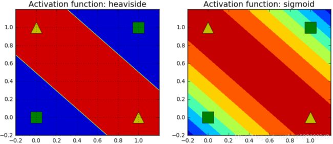
Figure 10-6. XOR classification problem and an MLP that solves it![]()
def sigmoid(z):
    return 1/(1+np.exp(-z)) # >0.5 ==> positive, <0.5 ==>negative

def heaviside(z):
    #if z>=0 ==>True ==>1 OR ==>False ==>0
    #arr = np.array([1,2,3,4,5])
    #(arr>=0).astype( arr.dtype ) ==> array([1, 1, 1, 1, 1])
    return (z>=0).astype(z.dtype) #>=0 ==> class #1, <0 ==> class #0

def mlp_xor(x1, x2, activation = heaviside):
    return activation( -1*activation( x1+x2-1.5 ) + activation( x1+x2-0.5 ) -0.5 )


x1s = np.linspace(-0.2, 1.2, 100)
x2s = np.linspace(-0.2, 1.2, 100)
x1, x2 = np.meshgrid(x1s, x2s)

z1 = mlp_xor(x1, x2, activation=heaviside)
z2 = mlp_xor(x1, x2, activation=sigmoid)

plt.figure( figsize=(10,4) )

plt.subplot(121)
plt.contourf(x1, x2, z1)
plt.plot([0,1], [0,1], "gs", markersize=20)
plt.plot([0,1], [1,0], "y^", markersize=20)
plt.title("Activation function: heaviside", fontsize=14)
plt.grid(True)

plt.subplot(122)
plt.contourf(x1, x2, z2)
plt.plot([0,1], [0,1], "gs", markersize=20)
plt.plot([0,1], [1,0], "y^", markersize=20)
plt.title("Activation function: sigmoid", fontsize=14)

plt.show()
However, it turns out that some of the limitations of Perceptrons can be eliminated by stacking multiple Perceptrons. The resulting ANN is called a Multi-Layer Perceptron (MLP). In particular, an MLP can solve the XOR problem, as you can verify by computing the output of the MLP represented on the right of Figure 10-6, for each combination of inputs: with inputs (0, 0) or (1, 1) the network outputs 0, and with inputs (0, 1) or (1, 0) it outputs 1. All connections have a weight equal to 1, except the four connections where the weight is shown. Try verifying that this network indeed solves the XOR problem!
The Multilayer Perceptron and Backpropagation(反向传播(B-P网络),可以用来表示一种神经网络算法)
Figure 10-7. Architecture of a Multilayer Perceptron with two inputs, one hidden layer of four neurons, and three output neurons (the bias neurons are shown here, but usually they are implicit内含的)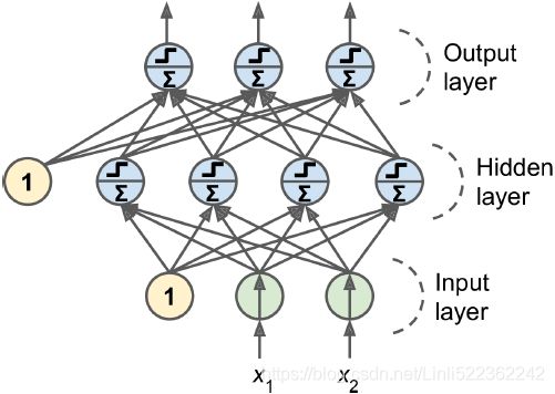
An MLP is composed of one (passthrough) input layer, one or more layers of TLUs, called hidden layers, and one final layer of TLUs called the output layer (see Figure 10-7). The layers close to the input layer are usually called the lower layers, and the ones close to the outputs are usually called the upper layers. Every layer except the output layer includes a bias neuron and is fully connected to the next layer.
######################################
The signal flows only in one direction (from the inputs to the outputs), so this architecture is an example of a feedforward neural network (FNN).
######################################
When an ANN contains a deep stack of hidden layers, it is called a deep neural network (DNN). The field of Deep Learning studies DNNs, and more generally models containing deep stacks of computations. Even so, many people talk about Deep Learning whenever neural networks are involved (even shallow ones).
For many years researchers struggled to find a way to train MLPs, without success. But in 1986, David Rumelhart, Geoffrey Hinton, and Ronald Williams published a From Biological groundbreaking paper that introduced the backpropagation反向传播(B-P网络) training algorithm, which is still used today. In short, it is Gradient Descent (introduced in https://blog.csdn.net/Linli522362242/article/details/104005906) using an efficient technique for computing the gradients automatically: in just two passes through the network (one forward, one backward), the backpropagation algorithm is able to compute the gradient of the network's error with regard to every single model parameter. In other words, it can find out how each connection weight and each bias term should be tweaked in order to reduce the error. Once it has these gradients, it just performs a regular Gradient Descent step, and the whole process is repeated until the network converges to the solution.
##########################
Automatically computing gradients is called automatic differentiation, or autodiff. There are various autodiff techniques, with different pros and cons. The one used by backpropagation is called reverse-mode autodiff. It is fast and precise, and is well suited when the function to differentiate has many variables (e.g., connection weights) and few outputs (e.g., one loss). If you want to learn more about autodiff, check out https://blog.csdn.net/Linli522362242/article/details/106290394.
##########################
Let's run through this algorithm in a bit more detail:
- It handles one mini-batch at a time (for example, containing 32 instances each), and it goes through the full training set multiple times. Each pass is called an epoch.
- Each mini-batch is passed to the network's input layer, which sends it to the first hidden layer. The algorithm then computes the output of all the neurons in this layer (for every instance in the mini-batch). The result is passed on to the next layer, its output is computed and passed to the next layer, and so on until we get the output of the last layer, the output layer. This is the forward pass: it is exactly like making predictions, except all intermediate results are preserved since they are needed for the backward pass.
- Next, the algorithm measures the network's output error (i.e., it uses a loss function that compares the desired output and the actual output of the network, and returns some measure of the error).
- Then it computes how much each output connection contributed to the error. This is done analytically by applying the chain rule (perhaps the most fundamental rule in calculus), which makes this step fast and precise.
- The algorithm then measures how much of these error contributions came from each connection in the layer below, again using the chain rule, working backward until the algorithm reaches the input layer. As explained earlier, this reverse pass efficiently measures the error gradient across all the connection weights in the network by propagating the error gradient backward through the network (hence the name of the algorithm).
- Finally, the algorithm performs a Gradient Descent step to tweak all the connection weights in the network, using the error gradients it just computed.
This algorithm is so important that it's worth summarizing it again: for each training instance, the backpropagation algorithm first makes a prediction (forward pass) and measures the error, then goes through each layer in reverse to measure the error contribution from each connection (reverse pass), and finally tweaks the connection weights to reduce the error (Gradient Descent step).
######################################
It is important to initialize all the hidden layers' connection weights randomly, or else training will fail. For example, if you initialize all weights and biases to zero, then all neurons in a given layer will be perfectly identical, and thus backpropagation will affect them in exactly the same way, so they will remain identical. In other words, despite having hundreds of neurons per layer, your model will act as if it had only one neuron per layer: it won't be too smart. If instead you randomly initialize the weights, you break the symmetry and allow backpropagation to train a diverse team of neurons.
######################################
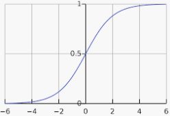
In order for this algorithm to work properly, its authors made a key change to the MLP's architecture: they replaced the step function with the logistic (sigmoid) function, σ(z) = 1 / (1 + exp(–z)). This was essential because the step function contains only flat segments, so there is no gradient to work with (Gradient Descent cannot move on a flat surface), while the logistic function has a well-defined nonzero derivative everywhere, allowing Gradient Descent to make some progress at every step. In fact, the backpropagation algorithm works well with many other activation functions, not just the logistic function. Here are two other popular choices:
- The hyperbolic双曲线的 tangent function tanh (z) = 2σ(2z) – 1 Just like the logistic function it is S-shaped, continuous, and differentiable, but its output value ranges from –1 to 1 (instead of 0 to 1 in the case of the logistic function), which tends to make each layer's output more or less normalized (i.e., centered around 0) at the beginning of training. This often helps speed up convergence.

The ReLU function (introduced in https://blog.csdn.net/Linli522362242/article/details/106325257) ReLU (z) = max (0, z). It is continuous but unfortunately not differentiable at z = 0 (the slope changes abruptly突然地, which can make Gradient Descent bounce around). However, in practice it works very well and has the advantage of being fast to compute. Most importantly, the fact that it does not have a maximum output value also helps reduce some issues during Gradient Descent (we will come back to this in Chapter 11).
These popular activation functions and their derivatives are represented in Figure 10-8. But wait! Why do we need activation functions in the first place? Well, if you chain several linear transformations, all you get is a linear transformation. For example, if f(x) = 2x + 3 and g(x) = 5x – 1, then chaining these two linear functions gives you another linear function: f(g(x)) = 2(5x – 1) + 3 = 10x + 1. So if you don't have some nonlinearity between layers, then even a deep stack of layers is equivalent to a single layer, and you can't solve very complex problems with that. Conversely, a large enough DNN with nonlinear activations can theoretically approximate any continuous function.
def sigmoid(z):
    return 1/(1+np.exp(-z))

def relu(z):
    return np.maximum( 0,z )

# Numerical Differentiation
# https://blog.csdn.net/Linli522362242/article/details/106290394
def derivative(f, z, eps=0.000001):
    # 1/2 * ( f(z+eps)-f(z)/eps + ( f(z)-f(z-eps) )/eps )
    # 1/2 * ( f(z+eps)/eps + f(z-eps)/eps )
    return ( f(z+eps) - f(z-eps) )/(2*eps)
z = np.linspace(-5, 5, 200)
plt.figure( figsize=(11,4) )
plt.subplot(121)
plt.plot( z, np.sign(z), "r-", linewidth=1, label="Step" )
plt.plot( z, sigmoid(z), "y--", linewidth=2, label="Sigmoid" )
plt.plot( z, np.tanh(z), "b-", linewidth=2, label="Tanh" )
plt.plot( z, relu(z), "k-.", linewidth=2, label="ReLU" ) #ReLU (z) = max (0, z)
plt.grid(True)
plt.legend( loc="center right", fontsize=14 )
plt.title("Activation function", fontsize=14 )
plt.axis([-5, 5, -1.2, 1.2])
plt.subplot(122)
plt.plot(z, derivative(np.sign, z), "r-", linewidth=1, label="Step")
plt.plot(0, 0, "ro", markersize=5)
plt.plot(0, 0, "rx", markersize=10)
plt.plot(z, derivative(sigmoid, z), "y--", linewidth=2, label="sigmoid")
plt.plot(z, derivative(np.tanh, z), "b-", linewidth=2, label="Tanh")
plt.plot(z, derivative( relu, z ), "k-.", linewidth=2, label="ReLU")
plt.grid(True)
plt.title("Derivatives", fontsize=14)
plt.axis([-5,5, -0.2, 1.2])
plt.show()![]()
OK! You know where neural nets came from, what their architecture is, and how to compute their outputs. You've also learned about the backpropagation algorithm. But what exactly can you do with them?
Regression MLPs
First, MLPs can be used for regression tasks. If you want to predict a single value (e.g., the price of a house, given many of its features), then you just need a single output neuron: its output is the predicted value. For multivariate regression (i.e., to predict multiple values at once), you need one output neuron per output dimension. For example, to locate the center of an object in an image, you need to predict 2D coordinates, so you need two output neurons. If you also want to place a bounding box around the object, then you need two more numbers: the width and the height of the object. So, you end up with four output neurons.
In general, when building an MLP for regression, you do not want to use any activation function for the output neurons, so they are free to output any range of values. If you want to guarantee that the output will always be positive, then you can use the ReLU activation function in the output layer. Alternatively, you can use the softplus
activation function, which is a smooth variant of ReLU: softplus(z) = log(1 + exp(z)). It is close to 0 when z is negative, and close to z when z is positive. Finally, if you want to guarantee that the predictions will fall within a given range of values, then you can use the logistic function or the hyperbolic tangent, and then scale the labels to the appropriate range: 0 to 1 for the logistic function and –1 to 1 for the hyperbolic tangent.
The loss function to use during training is typically the mean squared error, but if you have a lot of outliers in the training set, you may prefer to use the mean absolute error instead. Alternatively, you can use the Huber loss, which is a combination of both.
#############################
Note
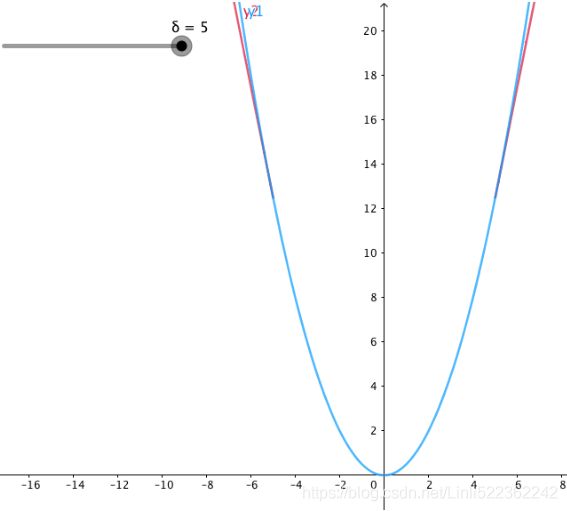
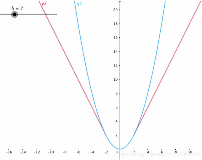
The Huber loss is quadratic when the error is smaller than a threshold δ (typically 1) but linear when the error is larger than δ. The linear part makes it less sensitive to outliers than the mean squared error, and the quadratic part allows it to converge faster and be more precise than the mean absolute error.
The Huber loss function describes the penalty incurred by an estimation procedure f. Huber (1964) defines the loss function piecewise by
This function is quadratic for small values of a, and linear for large values, with equal values and slopes of the different sections at the two points where ![]() . The variable a often refers to the residuals, that is to the difference between the observed and predicted values
. The variable a often refers to the residuals, that is to the difference between the observed and predicted values ![]() , so the former can be expanded to
, so the former can be expanded to ![]()
https://www.cnblogs.com/nowgood/p/Huber-Loss.html
Loss vs x for deferent value of ![]()
https://en.wikipedia.org/wiki/Huber_loss
#############################
Table 10-1 summarizes the typical architecture of a regression MLP.
Table 10-1. Typical regression MLP architecture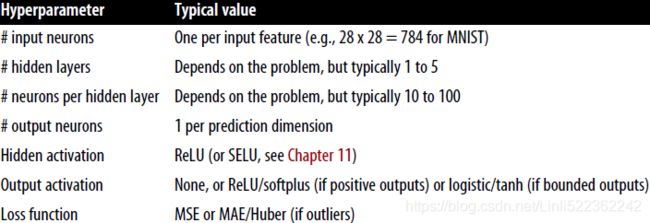
Classification MLPs
MLPs can also be used for classification tasks. For a binary classification problem, you just need a single output neuron using the logistic activation function: the output will be a number between 0 and 1, which you can interpret as the estimated probability of the positive class. The estimated probability of the negative class is equal to one minus that number.
MLPs can also easily handle multilabel binary classification tasks (see https://blog.csdn.net/Linli522362242/article/details/103786116). For example, you could have an email classification system that predicts whether each incoming email is ham or spam, and simultaneously predicts whether it is an urgent急迫的 or nonurgent email. In this case, you would need two output neurons, both using the logistic activation function: the first would output the probability that the email is spam, and the second would output the probability that it is urgent. More generally, you would dedicate one output neuron for each positive class. Note that the output probabilities do not necessarily add up to 1. This lets the model output any combination of labels: you can have nonurgent ham, urgent ham, nonurgent spam, and perhaps even urgent spam (although that would probably be an error).
If each instance can belong only to a single class, out of three or more possible classes (e.g., classes 0 through 9 for digit image classification), then you need to have one output neuron per class, and you should use the softmax activation function for the whole output layer (see Figure 10-9). The softmax function (introduced in https://blog.csdn.net/Linli522362242/article/details/104124771) will ensure that all the estimated probabilities are between 0 and 1 and that they add up to 1 (which is required if the classes are exclusive). This is called multiclass classification.
Figure 10-9. A modern MLP (including ReLU and softmax) for classification

Biological neurons seem to implement a roughly sigmoid (S-shaped) activation function, so researchers stuck to sigmoid functions for a very long time. But it turns out that the ReLU activation function generally works better in ANNs. This is one of the cases where the biological analogy was misleading.
Equation 4-19. Softmax score for class k ![]()
Equation 4-20. Softmax function ![]()
Equation 4-21. Softmax Regression classifier prediction ![]()
Equation 4-22. Cross entropy cost function ![]()
![]() is equal to 1 if the target class for the ith instance is k; otherwise, it is equal to 0.
is equal to 1 if the target class for the ith instance is k; otherwise, it is equal to 0.
Notice that when there are just two classes (K = 2), this cost function is equivalent to the Logistic Regression's cost function (log loss; see Equation 4-17 ![]()
![]() is a weight vector: Theta = Theta - eta*gradients
is a weight vector: Theta = Theta - eta*gradients
Regarding the loss function, since we are predicting probability distributions, the cross-entropy loss (also called the log loss, see https://blog.csdn.net/Linli522362242/article/details/104124771) is generally a good choice.
Table 10-2 summarizes the typical architecture of a classification MLP
########################
Before we go on, I recommend you go through exercise 1 at the end of this chapter. You will play with various neural network architectures and visualize their outputs using the TensorFlow Playground. This will be very useful to better understand MLPs, including the effects of all the hyperparameters (number of layers and neurons, activation functions, and more).
########################
https://docs.floydhub.com/guides/environments/
https://www.w3cschool.cn/tensorflow_python/tensorflow_python-4pyc2nuy.html
Training an MLP with TensorFlow's High-Level API
The simplest way to train an MLP with TensorFlow is to use the high-level API TF.Learn, which is quite similar to Scikit-Learn’s API. The DNNClassifier class makes it trivial to train a deep neural network with any number of hidden layers, and
a softmax output layer to output estimated class probabilities. For example, the following code trains a DNN for classification with two hidden layers (one with 300 neurons, and the other with 100 neurons) and a softmax output layer with 10 neurons:
import tensorflow as tfimport keras 问题签名:
问题事件名称: BEX64
应用程序名: python.exe
应用程序版本: 3.5.6150.1013
应用程序时间戳: 5b832238
故障模块名称: StackHash_1dc2
故障模块版本: 0.0.0.0
故障模块时间戳: 00000000
异常偏移: 0000000000000000
异常代码: c0000005
异常数据: 0000000000000008
OS 版本: 6.1.7601.2.1.0.256.1
区域设置 ID: 1033
其他信息 1: 1dc2
其他信息 2: 1dc22fb1de37d348f27e54dbb5278e7d
其他信息 3: cbc5
其他信息 4: cbc5ec6970b2af35927ad67117ca57e2
(suggestion: Restart your sytem OR close some application)
import tensorflow as tf
import keras ![]()
keras.__version__ ![]()
tf.__version__![]()
(X_train, y_train), (X_test, y_test) = keras.datasets.mnist.load_data()(X_train, y_train), (X_test, y_test) = keras.datasets.mnist.load_data()
X_train.shape ![]()
X_train[:2]X_train = X_train.astype( np.float32 )
X_train[:2] ![]()
X_train = X_train.astype( np.float32 ).reshape(-1, 28*28)
X_train.shape ![]()
(X_train, y_train), (X_test, y_test) = keras.datasets.mnist.load_data()
# the original dtype=unit8, now it will be converted to np.float32
X_train = X_train.astype( np.float32 ).reshape(-1, 28*28) / 255.0
X_test = X_test.astype( np.float32 ).reshape(-1, 28*28) /255.0
y_train = y_train.astype( np.int32 )
y_test = y_test.astype( np.int32 )

feature_cols = tf.contrib.learn.infer_real_valued_columns_from_input(X_train)
# hidden_units=[300,100]
# two hidden layers (one with 300 neurons, and the other with 100 neurons)
# n_classes=10 : a softmax output layer with 10 neurons
dnn_clf = tf.contrib.learn.DNNClassifier( hidden_units=[300,100], n_classes=10,
                                         feature_columns=feature_cols)
dnn_clf.fit(x=X_train, y=y_train, batch_size=50, steps=40000)
feature_cols = tf.contrib.learn.infer_real_valued_columns_from_input(X_train)
dnn_clf = tf.contrib.learn.DNNClassifier( hidden_units=[300,100], n_classes=10,
feature_columns=feature_cols)
dnn_clf.fit(x=X_train, y=y_train, batch_size=50, steps=40000)
... ...
If you run this code on the MNIST dataset (after scaling it, e.g., by using Scikit-Learn’s StandardScaler), you may actually get a model that achieves over 98.1% accuracy on the test set! That’s better than the best model we trained in https://blog.csdn.net/Linli522362242/article/details/103786116:
from sklearn.metrics import accuracy_score
y_pred = list(dnn_clf.predict(X_test))
accuracy_score(y_test, y_pred)
The TF.Learn library also provides some convenience functions to evaluate models:
dnn_clf_clf.evaluate( X_test, y_test) 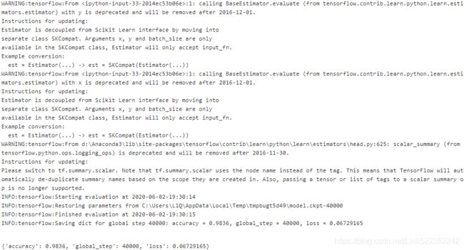
Under the hood, the DNNClassifier class creates all the neuron layers, based on the ReLU activation function (we can change this by setting the activation_fn hyperparameter). The output layer relies on the softmax function, and the cost function is cross entropy (introduced in https://blog.csdn.net/Linli522362242/article/details/104124771).
Another way of Training an MLP with TensorFlow's High-Level API
(X_train, y_train), (X_test, y_test) = keras.datasets.mnist.load_data()
# the original dtype=unit8, now it will be converted to np.float32
X_train = X_train.astype( np.float32 ).reshape(-1, 28*28) / 255.0
X_test = X_test.astype( np.float32 ).reshape(-1, 28*28) /255.0
y_train = y_train.astype( np.int32 )
y_test = y_test.astype( np.int32 )
X_valid, X_train = X_train[:5000], X_train[5000:]
y_valid, y_train = y_train[:5000], y_train[5000:]


feature_cols = [tf.feature_column.numeric_column("X", shape=[28*28])]
dnn_clf = tf.contrib.learn.DNNClassifier( hidden_units=[300,100], n_classes=10,
                                         feature_columns=feature_cols)
input_fn = tf.estimator.inputs.numpy_input_fn(x={"X":X_train}, y=y_train,
                                              num_epochs=40, batch_size=50, shuffle = True)
dnn_clf.fit(input_fn=input_fn)
feature_cols = [ tf.feature_column.numeric_column("X", shape=[28*28]) ]
dnn_clf = tf.contrib.learn.DNNClassifier( hidden_units=[300,100], n_classes=10,
feature_columns=feature_cols)
input_fn = tf.estimator.inputs.numpy_input_fn(x={"X":X_train}, y=y_train,
num_epochs=40, batch_size=50, shuffle = True)
dnn_clf.fit(input_fn=input_fn)
test_input_fn = tf.estimator.inputs.numpy_input_fn( x={"X":X_test}, y=y_test, shuffle=False )
eval_results = dnn_clf.evaluate( input_fn=test_input_fn )
eval_results ![]()
y_pred_iter = dnn_clf.predict(input_fn = test_input_fn)y_pred = list(y_pred_iter)
y_pred[0] ![]()
##############################################
The TF.Learn API is still quite new, so some of the names and functions used in these examples may evolve a bit by the time However, the general ideas should not change.
##############################################
Training a DNN Using Plain TensorFlow
If you want more control over the architecture of the network, you may prefer to use TensorFlow’s lower-level Python API (introduced in https://blog.csdn.net/Linli522362242/article/details/106214525). In this section we will build the same model as before using this API, and we will implement Minibatch Gradient Descent to train it on the MNIST dataset. The first step is the construction phase, building the TensorFlow graph. The second step is the execution phase, where you actually run the graph to train the model.
Construction Phase
Let's start. First we need to import the tensorflow library. Then we must specify the number of inputs and outputs, and set the number of hidden neurons in each layer:
import tensorflow as tf

n_inputs = 28*28 #MNIST
n_hidden1 = 300
n_hidden2 = 100
n_outputs = 10
Next, just like you did in https://blog.csdn.net/Linli522362242/article/details/106214525, you can use placeholder nodes to represent the training data and targets. The shape of X is only partially defined. We know that it will be a 2D tensor (i.e., a matrix), with instances along the first dimension and features along the second dimension, and we know that the number of features is going to be 28 x 28 (one feature per pixel), but we don't know yet how many instances each training batch will contain. So the shape of X is (None, n_inputs). Similarly, we know that y will be a 1D tensor with one entry per instance, but again we don't know the size of the training batch at this point, so the shape of y is (None).
tf.reset_default_graph()

X = tf.placeholder( tf.float32, shape=(None, n_inputs), name="X" )
y = tf.placeholder( tf.int32, shape=(None), name="y")
Now let's create the actual neural network. The placeholder X will act as the input layer; during the execution phase, it will be replaced with one training batch at a time (note that all the instances in a training batch will be processed simultaneously by the neural network).
Now you need to create the two hidden layers and the output layer. The two hidden layers are almost identical: they differ only by the inputs they are connected to and by the number of neurons they contain. The output layer is also
very similar, but it uses a softmax activation function instead of a ReLU activation function. So let’s create a neuron_layer() function that we will use to create one layer at a time. It will need parameters to specify the inputs, the number of neurons, the activation function, and the name of the layer:
Let's go through the following code line by line:
- First we create a name scope using the name of the layer: it will contain all the computation nodes for this neuron layer. This is optional, but the graph will look much nicer in TensorBoard if its nodes are well organized.
- Next, we get the number of inputs by looking up the input matrix’s shape and getting the size of the second dimension (the first dimension is for instances).

- The next three lines create a W variable that will hold the weights matrix. It will be a 2D tensor containing all the connection weights between each input and each neuron; hence, its shape will be (n_inputs, n_neurons). It will be initialized randomly, using a truncated normal (Gaussian) distribution with a standard deviation of
 (Using a truncated normal distribution rather than a regular normal distribution ensures that there won't be any large weights, which could slow down training. ### truncated_normal( shape, mean=0.0, stdev=1.0 ) # range: [ mean-2*stddev, mean+2*stddev ]###). Using this specific standard deviation helps the algorithm converge much faster (we will discuss this further in Chapter 11; it is one of those small tweaks to neural networks that have had a tremendous impact on their efficiency). It is important to initialize connection weights randomly for all hidden layers to avoid any symmetries that the Gradient Descent algorithm would be unable to break.
- The next line creates a b variable for biases, initialized to 0 (no symmetry issue in this case), with one bias parameter per neuron.
- Then we create a subgraph to compute z = X · W + b. This vectorized implementation will efficiently compute the weighted sums of the inputs plus the bias term for each and every neuron in the layer, for all the instances in the batch in just one shot.
- Finally, if the activation parameter is set to "relu", the code returns relu(z) (i.e., max (0, z)), or else it just returns z.
#inputs, the number of neurons, the name of the layer, the activation function
def neuron_layer( X, n_neurons, name, activation=None):
    with tf.name_scope(name):
        n_inputs = int( X.get_shape()[1] ) # X.get_shape()[1] : the number of features

        stddev = 2 / np.sqrt( n_inputs )
                                       # shape
        init = tf.truncated_normal( (n_inputs, n_neurons), stddev=stddev )
        # truncated_normal( shape, mean=0.0, stdev=1.0 ) # range: [ mean-2*stddev, mean+2*stddev ]
        # stddev=stddev ==> stddev= 2/np.sqrt( n_inputs ) ==> range: mean += 2* 2/np.sqrt( n_inputs )
        # 截断的产生正态分布的随机数,即随机数与均值的差值若大于两倍的标准差,则重新生成 |x-mean| <=2*stddev
        W = tf.Variable(init, name="kernel")
        b = tf.Variable(tf.zeros([n_neurons]), name="bias")
        Z = tf.matmul( X,W) # X dot W # prediction
        if activation is not None:
            return activation(Z)
        else:
            return Z
#n_inputs = 28*28 ==> n_hidden1 = 300 ==> n_hidden2 = 100 ==> n_outputs = 10
Okay, so now you have a nice function to create a neuron layer. Let's use it to create the deep neural network!
* The first hidden layer takes X as its input.
hidden1 = neuron_layer( X, n_hidden1, name="hidden1", activation=tf.nn.relu )
* The second takes the output of the first hidden layer as its input.
hidden2 = neuron_layer( hidden1, n_hidden2, name="hidden2", activation=tf.nn.relu )
* And finally, the output layer takes the output of the second hidden layer as its input.
logits = neuron_layer( hidden2, n_outputs, name="outputs" )
#n_inputs = 28*28+1 ==> n_hidden1 = 300 ==> n_hidden2 = 100 ==> n_outputs = 10
with tf.name_scope("dnn"):
    hidden1 = neuron_layer( X, n_hidden1, name="hidden1", activation=tf.nn.relu )
    hidden2 = neuron_layer( hidden1, n_hidden2, name="hidden2", activation=tf.nn.relu )
    logits = neuron_layer( hidden2, n_outputs, name="outputs" )
Notice that once again we used a name scope for clarity清晰度. Also note that logits is the output of the neural network before going through the softmax activation function: for optimization reasons, we will handle the softmax computation later.![]() ==>
==>![]() ==>
==>![]()
As you might expect, TensorFlow comes with many handy functions to create standard neural network layers, so there's often no need to define your own neuron_layer() function like we just did. For example, TensorFlow's fully_connected() function creates a fully connected layer, where all the inputs are connected to all the neurons in the layer. It takes care of creating the weights and biases variables, with the proper initialization strategy, and it uses the ReLU activation function by default (we can change this using the activation_fn argument). As we will see in Chapter 11, it also supports regularization and normalization parameters. Let's tweak the preceding code to use the fully_connected() function instead of our neuron_layer() function. Simply import the function and replace the dnn construction section with the following code:
from tensorflow.contrib.layers import fully_connected

with tf.name_scope("dnn"):
    hidden1 = fully_connected(X, n_hidden1, scope="hidden1")
    hidden2 = fully_connected(hidden1, n_hidden2, scope="hidden2")
    logits = fully_connected(hidden2, n_outputs, scope="outputs", activation_fn=None)
###################
The tensorflow.contrib package contains many useful functions, but it is a place for experimental code that has not yet graduated to be part of the main TensorFlow API. So the fully_connected() function (and any other contrib code) may change or move in the future.
###################
Now that we have the neural network model ready to go, we need to define the cost function that we will use to train it. Just as we did for Softmax Regression in Cp4 https://blog.csdn.net/Linli522362242/article/details/104124771, we will use cross entropy. As we discussed earlier, cross entropy will penalize models that estimate a low probability for the target class. TensorFlow provides several functions to compute cross entropy. We will use sparse_softmax_cross_entropy_with_logits(): it computes the cross entropy based on the “logits” (i.e., the output of the network before going through the softmax activation function), and it expects labels in the form of integers ranging from 0 to the number of classes minus 1 (in our case, from 0 to 9). This will give us a 1D tensor containing the cross entropy for each instance. We can then use TensorFlow's reduce_mean() function to compute the mean cross entropy over all instances.![]() ==>
==>![]() ==>
==>
Equation 4-22. Cross entropy cost function ![]()
![]() is equal to 1 if the target class for the ith instance is k; otherwise, it is equal to 0.
is equal to 1 if the target class for the ith instance is k; otherwise, it is equal to 0.
Notice that when there are just two classes (K = 2), this cost function is equivalent to the Logistic Regression's cost function (log loss; see Equation 4-17 ![]()
(Note: usually we are not using the term , but here we use it since the author's idea)
#Cross entropy cost function ![]() +
+ ![]()
an additional ![]() penalty:
penalty: ![]()
Then Cross entropy gradient vector for class k
![]() +
+ ![]() *
* ![]() (this equation also has to add a step for containing the case of i=0 for bias)
(this equation also has to add a step for containing the case of i=0 for bias)![]() is a weight vector: Theta = Theta - eta*gradients , eta is the learning rate
is a weight vector: Theta = Theta - eta*gradients , eta is the learning rate ![]()
with tf.name_scope("loss"):
    xentropy = tf.nn.sparse_softmax_cross_entropy_with_logits( labels=y, logits=logits )
    loss = tf.reduce_mean( xentropy, name="loss")
################################
The sparse_softmax_cross_entropy_with_logits() function is equivalent to applying the softmax activation function###![]() return index/k max of
return index/k max of ![]() ###and then computing the cross entropy(
###and then computing the cross entropy(![]() +
+ ![]() ), but it is more efficient, and it properly takes care of corner cases like logits equal to 0 (-infinity). This is why we did not apply the softmax activation function earlier(Now, you understand that "logits is the output of the neural network before going through the softmax activation function"). There is also another function called softmax_cross_entropy_with_logits(), which takes labels in the form of one-hot vectors (instead of ints from 0 to the number of classes minus 1).
), but it is more efficient, and it properly takes care of corner cases like logits equal to 0 (-infinity). This is why we did not apply the softmax activation function earlier(Now, you understand that "logits is the output of the neural network before going through the softmax activation function"). There is also another function called softmax_cross_entropy_with_logits(), which takes labels in the form of one-hot vectors (instead of ints from 0 to the number of classes minus 1).
https://blog.csdn.net/Linli522362242/article/details/104124771
to_one_hot(y_train[:10])![]()
################################
We have the neural network model, we have the cost function, and now we need to define a GradientDescentOptimizer that will tweak the model parameters to minimize the cost function. Nothing new; it’s just like we did in Cp9 https://blog.csdn.net/Linli522362242/article/details/106325257:
Then Cross entropy gradient![]() vector for class k
vector for class k
![]() +
+![]() *
*![]() (this euation also has to add a step for containing the case of i=0 for bias)
(this euation also has to add a step for containing the case of i=0 for bias)![]() is a weight vector: Theta = Theta - eta*gradients
is a weight vector: Theta = Theta - eta*gradients
# loss: Cross entropy cost function ![]() +
+ ![]()
https://blog.csdn.net/Linli522362242/article/details/106325257: Mini-batch GD with tensorflow
learning_rate = 0.01
with tf.name_scope("train"):
    optimizer = tf.train.GradientDescentOptimizer( learning_rate )
    training_op = optimizer.minimize(loss)
The last important step in the construction phase is to specify how to evaluate the model. We will simply use accuracy as our performance measure. First, for each instance, determine if the neural network's prediction is correct by checking whether or not the highest logit corresponds to the target class. For this you can use the in_top_k() function. This returns a 1D tensor full of boolean values (class predicted VS true class), so we need to cast these booleans to floats and then compute the average. This will give us the network’s overall accuracy.
with tf.name_scope("eval"):
    #k=1 is the top-one class  # tf.nn.in_top_k(predictions, targets, k, name=None)
    correct = tf.nn.in_top_k( logits, y, 1) #logits.shape : (samples, class_dimensions)
    accuracy = tf.reduce_mean( tf.cast(correct, tf.float32) )
And, as usual, we need to create a node to initialize all variables, and we will also create a Saver to save our trained model parameters to disk:
init = tf.global_variables_initializer()
saver = tf.train.Saver()
Phew! This concludes the construction phase. This was fewer than 40 lines of code, but it was pretty intense: we created placeholders for the inputs and the targets, we created a function to build a neuron layer, we used it to create the DNN, we defined the cost function, we created an optimizer, and finally we defined the performance measure. Now on to the execution phase.
Execution Phase
This part is much shorter and simpler.
First, let's load MNIST. We could use Scikit-Learn for that as we did in previous chapters, but TensorFlow offers its own helper that fetches the data, scales it (between 0 and 1), shuffles it, and provides a simple function to load one mini-batches a time. So let's use it instead:
from tensorflow.examples.tutorials.mnist import input_data

mnist = input_data.read_data_sets("/tmp/data/")
#from tensorflow.examples.tutorials.mnist import input_data
# mnist = input_data.read_data_sets("/tmp/data/")
import keras
(X_train, y_train), (X_test, y_test) = keras.datasets.mnist.load_data()
X_train = X_train.astype(np.float32).reshape(-1, 28*28) / 255.0
X_test = X_test.astype(np.float32).reshape(-1, 28*28) / 255.0
y_train = y_train.astype(np.int32)
y_test = y_test.astype(np.int32)
X_valid, X_train = X_train[:5000], X_train[5000:]
y_valid, y_train = y_train[:5000], y_train[5000:]Now we define the number of epochs that we want to run, as well as the size of the mini-batches:
n_epochs = 40
batch_size = 50
def shuffle_batch( X, y, batch_size ):
rnd_idx = np.random.permutation( len(X) )
n_batches = len(X) // batch_size
# np.array_split(rnd_idx, n_batches) # split the list of rnd_idx to n_batches groups
for batch_idx in np.array_split(rnd_idx, n_batches):
X_batch, y_batch = X[batch_idx], y[batch_idx]
yield X_batch, y_batchAnd now we can train the model:
# with tf.name_scope("loss"):                                    ########
#     xentropy = tf.nn.sparse_softmax_cross_entropy_with_logits( labels=y, logits=logits )
#     loss = tf.reduce_mean( xentropy, name="loss")

# learning_rate = 0.01
# with tf.name_scope("train"):
#     optimizer = tf.train.GradientDescentOptimizer( learning_rate )
#     training_op = optimizer.minimize(loss)

with tf.Session() as sess:
    init.run()
    for epoch in range(n_epochs):
        for X_batch, y_batch in shuffle_batch( X_train, y_train, batch_size ):
            sess.run(training_op, feed_dict={X: X_batch, y:y_batch})
        # Next, at the end of each epoch, the code evaluates the model on the last mini-batch
        # and on the full validation set, and it prints out the result.
        acc_batch = accuracy.eval(feed_dict={X: X_batch, y:y_batch})
        acc_val = accuracy.eval( feed_dict={X: X_valid, y: y_valid} )
        print( epoch, "(Last) Batch accuracy: ", acc_batch, "~ Val accuracy: ", acc_val )
save_path = saver.save(sess, "./my_model_final.ckpt") 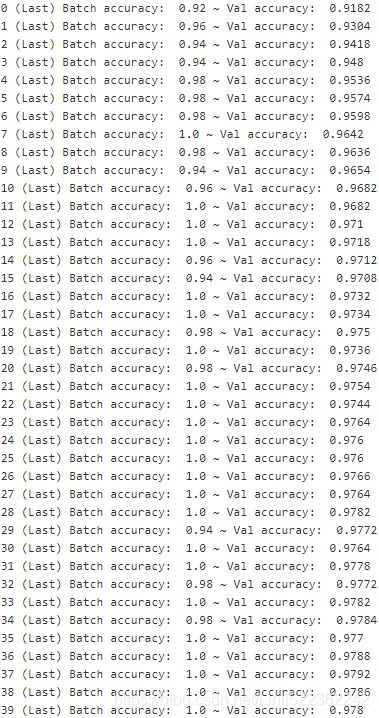
![]()
This code opens a TensorFlow session, and it runs the init node that initializes all the variables. Then it runs the main training loop: at each epoch, the code iterates through a number of mini-batches that corresponds to the training set size. Each mini-batch is fetched via the next_batch() method, and then the code simply runs the training operation, feeding it the current mini-batch input data and targets. Next, at the end of each epoch, the code evaluates the model on the last mini-batch and on the full validation set, and it prints out the result. Finally, the model parameters are saved to disk.
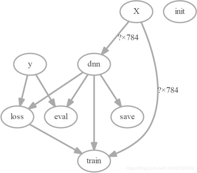
import tfgraphviz as tfg

tfg.board( tf.get_default_graph() ).view()ExecutableNotFound: failed to execute ['dot', '-Tpdf', '-O', 'G.gv'], make sure the Graphviz executables are on your systems' PATH
Solution:
import os
os.environ["PATH"] += os.pathsep + "D:/Graphviz2.38/bin" # " directory" where you intall graphviz

import tfgraphviz as tfg

tfg.board( tf.get_default_graph() ).view()
'G.gv.pdf'
Using the Neural Network
Now that the neural network is trained, you can use it to make predictions. To do that, you can reuse the same construction phase, but change the execution phase like this:
with tf.Session() as sess:
    saver.restore( sess, "./my_model_final.ckpt" ) # or better, use save_path
    X_new_scaled = X_test[:20]
    Z = logits.eval( feed_dict={X: X_new_scaled } )
    y_pred = np.argmax( Z, axis=1 )
INFO:tensorflow:Restoring parameters from ./my_model_final.ckpt
Z.shape![]() # 20 instences, 10 output classes' probabilities (a softmax output layer with 10 neurons )
# 20 instences, 10 output classes' probabilities (a softmax output layer with 10 neurons )
Z[:3]array([[ -0.94117993, -0.30440024, 3.7903986 , 6.0553164 ,
-4.243604 , 0.49758205, -8.51664 , 13.871222 ,
1.0109882 , 2.8417473 ],
[ 1.3493837 , 5.7800503 , 16.594517 , 7.134079 ,
-7.525274 , 3.8381264 , 0.93146825, -10.110606 ,
3.5289195 , -10.417238 ],
[ -2.9818027 , 9.603735 , 1.8501127 , -0.9166389 ,
0.58449167, -1.4478357 , -1.0345508 , 3.4288523 ,
1.1301693 , -1.9527786 ]], dtype=float32)
print("Predict classes: ", y_pred)
print("Actual classes:  ", y_test[:20])
Predict classes: [7 2 1 0 4 1 4 9 5 9 0 6 9 0 1 5 9 7 3 4]
Actual classes: [7 2 1 0 4 1 4 9 5 9 0 6 9 0 1 5 9 7 3 4]
First the code loads the model parameters from disk. Then it loads some new images that you want to classify. Remember to apply the same feature scaling as for the training data (in this case, scale it from 0 to 1). Then the code evaluates the logits node. If you wanted to know all the estimated class probabilities, you would need to apply
the softmax()###![]() ### function to the logits, but if you just want to predict a class, you can simply pick the class that has the highest logit value (using the argmax() function does the trick).
### function to the logits, but if you just want to predict a class, you can simply pick the class that has the highest logit value (using the argmax() function does the trick).![]()
( np.exp( Z ) / np.sum(np.exp( Z ), axis=0, keepdims=True) )[:3] # softmax equationarray([[1.1635773e-08, 3.3828209e-07, 2.7491981e-06, 2.5569927e-03,
1.2015606e-08, 3.7241718e-06, 3.5421127e-10, 2.9083505e-02,
1.1664371e-03, 1.0365442e-06],
[1.1496731e-07, 1.4849857e-04, 9.9991691e-01, 7.5202123e-03,
4.5137211e-10, 1.0515010e-04, 4.4928665e-06, 1.1180759e-12,
1.4467216e-02, 1.8083545e-12],
[1.5120426e-09, 6.7971586e-03, 3.9495768e-07, 2.3979919e-06,
1.5016237e-06, 5.3228661e-07, 6.2906037e-07, 8.4836631e-07,
1.3140774e-03, 8.5773220e-09]], dtype=float32)Fine-Tuning Neural Network Hyperparameters
The flexibility of neural networks is also one of their main drawbacks: there are many hyperparameters to tweak. Not only can you use any imaginable network topology (how neurons are interconnected), but even in a simple MLP you can change the number of layers, the number of neurons per layer, the type of activation function to use in each layer, the weight initialization logic, and much more. How do you know what combination of hyperparameters is the best for your task?
Of course, you can use grid search with cross-validation to find the right hyperparameters, like you did in previous chapters, but since there are many hyperparameters to tune, and since training a neural network on a large dataset takes a lot of time, you will only be able to explore a tiny part of the hyperparameter space in a reasonable amount of time. It is much better to use randomized search, as we discussed in Cp2 https://blog.csdn.net/Linli522362242/article/details/103646927. Another option is to use a tool such as Oscar, which implements more complex algorithms to help you find a good set of hyperparameters quickly.
It helps to have an idea of what values are reasonable for each hyperparameter, so you can restrict the search space. Let's start with the number of hidden layers.
Number of Hidden Layers
For many problems, you can just begin with a single hidden layer and you will get reasonable results. It has actually been shown that an MLP with just one hidden layer can model even the most complex functions provided it has enough neurons. For a long time, these facts convinced researchers that there was no need to investigate any deeper neural networks. But they overlooked the fact that deep networks have a much higher parameter efficiency than shallow ones: they can model complex functions using exponentially fewer neurons than shallow nets, making them much faster to train.
To understand why, suppose you are asked to draw a forest using some drawing software, but you are forbidden to use copy/paste. You would have to draw each tree individually, branch per branch, leaf per leaf.
If you could instead draw one leaf, copy/paste it to draw a branch, then copy/paste that branch to create a tree, and
finally copy/paste this tree to make a forest, you would be finished in no time. Realworld data is often structured in such a hierarchical way and DNNs automatically take advantage of this fact: lower hidden layers model low-level structures (e.g., line segments of various shapes and orientations), intermediate hidden layers combine these low-level structures to model intermediate-level structures (e.g., squares, circles), and the highest hidden layers and the output layer combine these intermediate structures to model high-level structures (e.g., faces).
Not only does this hierarchical architecture help DNNs converge faster to a good solution, it also improves their ability to generalize to new datasets. For example, if you have already trained a model to recognize faces in pictures, and you now want to train a new neural network to recognize hairstyles, then you can kickstart training by reusing the lower layers of the first network. Instead of randomly initializing the weights and biases of the first few layers of the new neural network, you can initialize them to the value of the weights and biases of the lower layers of the first network.
This way the network will not have to learn from scratch all the low-level structures that occur in most pictures; it will only have to learn the higher-level structures (e.g., hairstyles).
In summary, for many problems you can start with just one or two hidden layers and it will work just fine (e.g., you can easily reach above 97% accuracy on the MNIST dataset using just one hidden layer with a few hundred neurons, and above 98% accuracy using two hidden layers with the same total amount of neurons, in roughly the
same amount of training time). For more complex problems, you can gradually ramp up the number of hidden layers, until you start overfitting the training set. Very complex tasks, such as large image classification or speech recognition, typically require networks with dozens of layers (or even hundreds, but not fully connected ones, as we will see in Chapter 13), and they need a huge amount of training data. However, you will rarely have to train such networks from scratch: it is much more common to reuse parts of a pretrained state-of-the-art network that performs a similar task. Training will be a lot faster and require much less data (we will discuss this in Chapter 11).
Number of Neurons per Hidden Layer
Obviously the number of neurons in the input and output layers is determined by the type of input and output your task requires. For example, the MNIST task requires 28 x 28 = 784 input neurons and 10 output neurons. As for the hidden layers, a common practice is to size them to form a funnel [ˈfʌnəl] 漏斗, with fewer and fewer neurons at each layer—the rationale being that many low-level features can coalesce [ˌkoʊəˈles] 合并 into far fewer high-level features. For example, a typical neural network for MNIST may have two hidden layers, the first with 300 neurons and the second with 100. However, this practice is not as common now, and you may simply use the same size for all hidden layers—for example, all hidden layers with 150 neurons: that's just one hyperparameter to tune instead of one per layer. Just like for the number of layers, you can try increasing the number of neurons gradually until the network starts overfitting. In general you will get more bang for the buck by increasing the number of layers than the number of neurons per layer. Unfortunately, as you can see, finding the perfect amount of neurons is still somewhat of a black art.
A simpler approach is to pick a model with more layers and neurons than you actually need, then use early stopping to prevent it from overfitting (and other regularization techniques, especially dropout, as we will see in Chapter 11). This has been dubbed the “stretch pants” approach:12 instead of wasting time looking for pants tha perfectly match your size, just use large stretch pants that will shrink down to the right size.
Activation Functions
In most cases you can use the ReLU activation function in the hidden layers (or one of its variants, as we will see in Chapter 11). It is a bit faster to compute than other activation functions, and Gradient Descent does not get stuck as much on plateaus高原[plæˈtoʊz]局部最高点, thanks to the fact that it does not saturate for large input values (as opposed to the logistic function or the hyperbolic tangent function, which saturate at 1).
For the output layer, the softmax activation function is generally a good choice for classification tasks (when the classes are mutually exclusive). For regression tasks, you can simply use no activation function at all.
This concludes this introduction to artificial neural networks. In the following chapters, we will discuss techniques to train very deep nets, and distribute training across multiple servers and GPUs. Then we will explore a few other popular neural network architectures: convolutional neural networks卷积神经网络, recurrent neural networks循环神经网络, and autoencoders自动编码器.
#######################################
for tensorflow version '2.1.0' and keras '2.2.4-tf'
import tensorflow as tf
from tensorflow import keras

tf.__version__, keras.__version__ ![]()
from tensorflow.keras.datasets import mnist

(X_train, y_train), (X_test, y_test) = mnist.load_data()
X_train.shape ![]()
y_train![]()
X_test.shape, y_test ![]()
#######################################
10_Introduction to Artificial Neural Networks with Keras 2
https://blog.csdn.net/Linli522362242/article/details/106537459
Classifying movie reviews: a binary classification example
for tensorflow version '2.1.0' and keras '2.2.4-tf'
Two-class classification, or binary classification, may be the most widely applied kind of machine-learning problem. In this example, you’ll learn to classify movie reviews as positive or negative, based on the text content of the reviews.
The IMDB dataset
You’ll work with the IMDB dataset: a set of 50,000 highly polarized两极分化 reviews from the Internet Movie Database. They’re split into 25,000 reviews for training and 25,000 reviews for testing, each set consisting of 50% negative and 50% positive reviews.
Why use separate training and test sets? Because you should never test a machinelearning model on the same data that you used to train it! Just because a model performs well on its training data doesn’t mean it will perform well on data it has never seen; and what you care about is your model’s performance on new data (because you already know the labels of your training data—obviously you don’t need your model to predict those). For instance, it’s possible that your model could end up merely memorizing a mapping between your training samples and their targets, which would be useless for the task of predicting targets for data the model has never seen before. We’ll go over this point in much more detail in the next chapter.
Just like the MNIST dataset, the IMDB dataset comes packaged with Keras. It has already been preprocessed: the reviews (sequences of words) have been turned into sequences of integers, where each integer stands for a specific word in a dictionary.
The following code will load the dataset (when you run it the first time, about 80 MB of data will be downloaded to your machine).
Loading the IMDB dataset
from tensorflow.keras.datasets import imdb

( X_train, y_train), (X_test, y_test) = imdb.load_data( num_words=10000 ) ![]()
The argument num_words=10000 means you’ll only keep the top 10,000 most frequently occurring words in the training data. Rare words will be discarded. This allows you to work with vector data of manageable可管理的 size.
The variables train_data and test_data are lists of reviews; each review is a list of word indices (encoding a sequence of words). train_labels and test_labels are lists of 0s and 1s, where 0 stands for negative and 1 stands for positive:
train_data.shape, test_data.shape ![]()
train_data(samples, indices of words)
print( train_data[0] )train_labels[0]![]()
Because you’re restricting yourself to the top 10,000 most frequent words, no word index will exceed 10,000:
max( [max(sequence) for sequence in train_data] )![]()
For kicks, here’s how you can quickly decode one of these reviews back to English words:
# word_index is a dictionary mapping  each word to an integer index.
word_index = imdb.get_word_index()
print([ (word, index) for (word, index) in word_index.items() ][:3])![]()
#Reverses it, mapping every integer index to a word
                                            # key, value
reverse_word_index = dict([ (index, word) for (word, index) in word_index.items() ])
print( [ (index, word) for (index, word) in reverse_word_index.items() ][:3] )
[(34701, 'fawn'), (52006, 'tsukino'), (52007, 'nunnery')]Preparing the data
You can’t feed lists of integers into a neural network. You have to turn your lists(train_data and test_data) into tensors. There are two ways to do that:
- Pad your lists so that they all have the same length, turn them into an integer tensor of shape (samples, word_indices), and then use as the first layer in your network a layer capable of handling such integer tensors (the Embedding layer, which we’ll cover in detail later ).
- One-hot encode your lists to turn them into vectors of 0s and 1s. This would mean, for instance, turning the sequence [3, 5] into a 10,000-dimensional vector that would be all 0s except for indices 3 and 5, which would be 1s. Then you could use as the first layer in your network a Dense layer, capable of handling floating-point vector data.
Encoding the integer sequences into a binary matrix
import numpy as np

#sequences.shape==(samples, indices of words))
def vectorize_sequences( sequences, dimension=10000):
    results = np.zeros( (len(sequences), dimension) )
    for i, sequence in enumerate(sequences):
        #Set the position corresponding to the index of word in each sample to 1.0
        results[i, sequence] =1.
    return results

x_train = vectorize_sequences( train_data )
x_test = vectorize_sequences( test_data )
Here’s what the samples look like now:
print(x_train[0]) ![]()
You should also vectorize your labels, which is straightforward:
train_labels.dtype![]()
# convert the dataset to array then
# give the dense layer the ability to handle floating-point vector data
y_train = np.asarray(train_labels).astype('float32')
y_test = np.asarray(test_labels).astype('float32')
y_train![]()
Now the data is ready to be fed into a neural network.
Building your network
The input data is vectors, and the labels are scalars (1s and 0s): this is the easiest setup you’ll ever encounter. A type of network that performs well on such a problem is a simple stack of fully connected (Dense) layers with relu activations![]() : Dense(16, activation='relu').
: Dense(16, activation='relu').
The argument being passed to each Dense layer (16) is the number of hidden units of the layer. A hidden unit is a dimension in the representation space of the layer. each such Dense layer with a relu activation implements the following chain of tensor operations:![]()
model.add(layers.Dense(16, activation='relu', input_shape=(10000,)))Having 16 hidden units means the weight matrix W will have shape (input_dimension, 16): the dot product with W will project the input data onto a 16-dimensional representation space (and then you’ll add the bias vector b and apply the relu operation). You can intuitively understand the dimensionality of your representation space as “how much freedom you’re allowing the network to have when learning internal representations.” Having more hidden units (a higher-dimensional representation space) allows your network to learn more-complex representations, but it makes the network more computationally expensive and may lead to learning unwanted patterns (patterns that will improve performance on the training data but not on the test data).
There are two key architecture decisions to be made about such a stack of Dense layers:
- How many layers to use
- How many hidden units to choose for each layer
For the time being, you’ll have to trust me with the following architecture choice:
- Two intermediate layers with 16 hidden units each
- A third layer that will output the scalar prediction regarding the sentiment of the current review
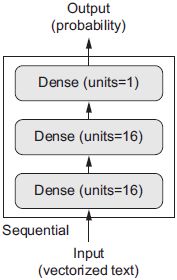
The intermediate layers will use relu as their activation function, and the final layer will use a sigmoid activation so as to output a probability (a score between 0 and 1, indicating how likely the sample is to have the target “1”: how likely the review is to be positive). A relu (rectified linear unit) is a function meant to zero out negative values (see figure 3.4), whereas a sigmoid “squashes” arbitrary values into the [0, 1] interval (see figure 3.5), outputting something that can be interpreted as a probability. Figure 3.4 The rectified linear unit function
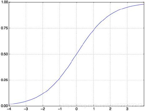 Figure 3.5 The sigmoid function
-
def sigmoid(z):
    return 1/(1+np.exp(-z))
here’s the Keras implementation, similar to the MNIST example you saw previously.
The model definition
from tensorflow import keras
import tensorflow as tf

tf.random.set_seed(42)

model = keras.models.Sequential()
model.add( keras.layers.Dense(16, activation = "relu", input_shape = (10000,)) ) #10000 dimensions
model.add( keras.layers.Dense(16, activation = "relu") )
model.add( keras.layers.Dense(1, activation="sigmoid") )
Guessing
First of all, this problem is a binary classification problem, which also contains 10,000 dimensions (or 100,000 feature variables). Machine learning is usually to find its most important features. The method used here is to gradually decrease the number of neurons of each hidden layer. and use the activation function to map to a high dimension space, and then easy to classify;
Since we are using the "relu" activation function, the value obtained is (0, max(z)). In addition, in order to minimize the error between the predicted value and the true value, or to find a closed solution (usually through derivation, it is a problem to find a closed form solution (OR to find the minimum value), its equation needs to be derivable (so the optional ones are sigmoid and Tanh), but consider the range of values for relu, so the best is to use sigmoid without negative value.
###########################
What are activation functions, and why are they necessary?
Without an activation function like relu (also called a non-linearity), the Dense layer would consist of two linear operations—a dot product and an addition: output = dot(W, input) + b
So the layer could only learn linear transformations (affine transformations仿射变换) of the input data: the hypothesis space of the layer would be the set of all possible linear transformations of the input data into a 16-dimensional space. Such a hypothesis space(Without an activation function) is too restricted and wouldn’t benefit from multiple layers of representations, because a deep stack of linear layers would still implement a linear operation: adding more layers wouldn’t extend the hypothesis space.
In order to get access to a much richer hypothesis space that would benefit from deep representations, you need a non-linearity, or activation function. relu is the most popular activation function in deep learning, but there are many other candidates, which all come with similarly strange names: prelu, elu, and so on.
###########################
Finally, you need to choose a loss function and an optimizer. Because you’re facing a binary classification problem and the output of your network is a probability (you end your network with a single-unit layer with a sigmoid activation), it’s best to use the binary_crossentropy loss. It isn’t the only viable choice: you could use, for instance, mean_squared_error. But crossentropy is usually the best choice when you’re dealing with models that output probabilities. Crossentropy is a quantity from the field of Information Theory that measures the distance between probability distributions or, in this case, between the ground-truth distribution and your predictions.
Here’s the step where you configure the model with the rmsprop optimizer and the binary_crossentropy loss function. Note that you’ll also monitor accuracy during training.
Compiling the model
model.compile( optimizer='rmsprop', loss='binary_crossentropy', metrics=['accuracy'] )You’re passing your optimizer, loss function, and metrics as strings, which is possible because rmsprop, binary_crossentropy, and accuracy are packaged as part of Keras.
Sometimes you may want to configure the parameters of your optimizer or pass a custom loss function or metric function. The former can be done by passing an optimizer class instance as the optimizer argument.
Configuring the optimizer
from tensorflow.keras import optimizers

model.compile( optimizer=optimizers.RMSprop(lr=0.001), loss='binary_crossentropy', metrics=['accuracy'] )
the latter can be done by passing function objects as the loss and/or metrics arguments,
model.compile( optimizer=optimizers.RMSprop(lr=0.001),
              loss=keras.losses.binary_crossentropy,
              metrics=[keras.metrics.binary_accuracy] )
Validating your approach
In order to monitor during training the accuracy of the model on data it has never seen before, you’ll create a validation set by setting apart 10,000 samples from the original training data.
Setting aside a validation set
x_val = x_train[:10000]
x_train_partial = x_train[10000:]
y_val = y_train[:10000]
y_train_partial = y_train[10000:]

print( x_val.shape,x_train.shape )![]()
You’ll now train the model for 20 epochs (20 iterations over all samples in the x_train and y_train tensors), in mini-batches of 512 samples. At the same time, you’ll monitor loss and accuracy on the 10,000 samples that you set apart(x_val). You do so by passing the validation data as the validation_data argument.
Training your model
model.compile( optimizer='rmsprop', loss='binary_crossentropy', metrics=['acc'] )
history = model.fit( x_train_partial, y_train_partial, epochs=20, batch_size=512, validation_data=(x_val, y_val) )On CPU, this will take less than 2 seconds per epoch—training is over in 20 seconds. At the end of every epoch, there is a slight pause as the model computes its loss and accuracy on the 10,000 samples of the validation data.
Note that the call to model.fit() returns a History object. This object has a member history, which is a dictionary containing data about everything that happened during training. Let’s look at it:
history_dict = history.history
history_dict.keys()![]()
The dictionary contains four entries条目: one per metric that was being monitored during training and during validation. In the following two listing, let’s use Matplotlib to plot the training and validation loss side by side (see figure 3.7), as well as the training and validation accuracy (see figure 3.8). Note that your own results may vary slightly due to a different random initialization of your network.
Plotting the training and validation loss
import matplotlib.pyplot as plt

history_dict = history.history
loss_values = history_dict['loss'] #train_loss
val_loss_values = history_dict['val_loss']

epochs = range(1, len(loss_values)+1) # [1~20]

plt.plot(epochs, loss_values, 'bo', label="Training_loss")
plt.plot(epochs, val_loss_values, 'b-', label='Validation loss' )
plt.title('Figure3.7 Training and validation loss')
plt.xlabel('Epochs')
plt.ylabel('Loss')
plt.legend()

plt.show()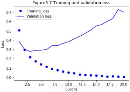
Plotting the training and validation accuracy
plt.clf()  #Clears the figure

acc_values = history_dict['acc']
val_acc_values = history_dict['val_acc']
plt.plot(epochs, acc_values, 'bo', label="Training acc")
plt.plot(epochs, val_acc_values, 'b-', label='Validation acc')
plt.title('Figure 3.8 Training and validation accuracy')
plt.xlabel('Epochs')
plt.ylabel('Loss')
plt.legend()

plt.show()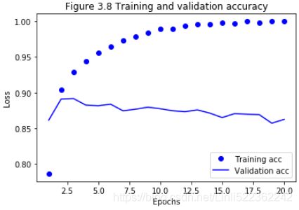
As you can see, the training loss decreases with every epoch, and the training accuracy increases with every epoch. That’s what you would expect when running gradient descent optimization—the quantity you’re trying to minimize should be less with every iteration. But that isn’t the case for the validation loss and accuracy: they seem to peak at the 3th epoch. This is an example of what we warned against earlier: a model that performs better on the training data isn’t necessarily a model that will do better on data it has never seen before. In precise terms, what you’re seeing is overfitting: after the second epoch, you’re overoptimizing on the training data, and you end up learning representations that are specific to the training data and don’t generalize to data outside of the training set.
In this case, to prevent overfitting, you could stop training after three epochs. In general, you can use a range of techniques to mitigate使减轻 overfitting.
Let’s train a new network from scratch for four epochs and then evaluate it on the test data.
Retraining a model from scratch
tf.random.set_seed(42)

model = keras.models.Sequential()
model.add( keras.layers.Dense(16, activation='relu', input_shape=(10000,)) ) #(batch_size, input_dim==10000)
model.add( keras.layers.Dense(16, activation='relu') )
model.add( keras.layers.Dense(1, activation='sigmoid') )

model.compile( optimizer='rmsprop', loss='binary_crossentropy', metrics=['accuracy'] )
model.fit(x_train, y_train, epochs=4, batch_size=512) #(batch_size, 10000)
results=model.evaluate(x_test, y_test)
The final results are as follows:
results![]()
This fairly naive approach achieves an accuracy of 88%. With state-of-the-art最先进的 approaches, you should be able to get close to 95%.
Using a trained network to generate predictions on new data
After having trained a network, you’ll want to use it in a practical setting. You can generate the likelihood of reviews being positive by using the predict method:
model.predict(x_test)Further experiments
The following experiments will help convince you that the architecture choices you’ve made are all fairly reasonable, although there’s still room for improvement:
- You used two hidden layers. Try using one or three hidden layers, and see how doing so affects validation and test accuracy.
- Try using layers with more hidden units or fewer hidden units: 32 units, 64 units, and so on.(may improve the performance~accuracy and more time cost)
- Try using the mse loss function instead of binary_crossentropy(similar).
- Try using the tanh activation (an activation that was popular in the early days of neural networks) instead of relu.
Wrapping up
Here’s what you should take away from this example:
- You usually need to do quite a bit of preprocessing on your raw data in order to be able to feed it—as tensors—into a neural network. Sequences of words can be encoded as binary vectors, but there are other encoding options, too.
- Stacks of Dense layers with relu activations can solve a wide range of problems (including sentiment情绪 classification), and you’ll likely use them frequently.
- In a binary classification problem (two output classes), your network should end with a Dense layer with one unit and a sigmoid activation: the output of your network should be a scalar between 0 and 1, encoding a probability.
- With such a scalar sigmoid output on a binary classification problem, the loss function you should use is binary_crossentropy.
- The rmsprop optimizer is generally a good enough choice, whatever your problem. That’s one less thing for you to worry about.
- As they get better on their training data, neural networks eventually start overfitting and end up obtaining increasingly worse results on data they’ve never seen before. Be sure to always monitor performance on data that is outside of the training set.
Classifying newswires新闻: a multiclass classification example
In the previous section, you saw how to classify vector inputs into two mutually exclusive classes using a densely connected neural network. But what happens when you have more than two classes?
In this section, you’ll build a network to classify Reuters(英国)路透社 newswires into 46 mutually exclusive topics. Because you have many classes, this problem is an instance of multiclass classification; and because each data point should be classified into only one category,
the problem is more specifically an instance of single-label, multiclass classification. If each data point could belong to multiple categories (in this case, topics), you’d be facing a multilabel, multiclass classification problem.
The Reuters dataset
You’ll work with the Reuters dataset, a set of short newswires and their topics, published by Reuters in 1986. It’s a simple, widely used toy dataset for text classification. There are 46 different topics; some topics are more represented than others, but each topic has at least 10 examples in the training set.
Like IMDB and MNIST, the Reuters dataset comes packaged as part of Keras. Let’s take a look.
from tensorflow.keras.datasets import reuters

(train_data, train_labels), (test_data, test_labels) = reuters.load_data(num_words=10000)![]()
As with the IMDB dataset, the argument num_words=10000 restricts the data to the 10,000 most frequently occurring words found in the data.
You have 8,982 training examples and 2,246 test examples:
train_data.shape, test_data.shape![]()
As with the IMDB reviews, each example is a list of integers (word indices):
print( train_data[10] )![]()
Here’s how you can decode it back to words, in case you’re curious.
Decoding newswires back to text
word_index = reuters.get_word_index()
reverse_word_index = dict([ (index,word) for (word, index) in word_index.items() ])
print( [ (index,word) for (index, word) in reverse_word_index.items() ][:3] )
# Note that the indices are offset by 3 because 0, 1, and 2 are reserved indices for “padding,” “start of sequence,”
# and “unknown.”
decoded_newswire = ' '.join( [reverse_word_index.get(i-3, '?') for i in train_data[0]] )
decoded_newswireThe label associated with an example is an integer between 0 and 45—a topic index:
import numpy as np
np.unique( train_labels )
Preparing the data
You can vectorize the data with the exact same code as in the previous example.
Encoding the data(since num_words=10000 restricts the data to the 10,000 most frequently occurring words found in the data)
def vectorize_sequences( sequences, dimensions=10000 ):
    results = np.zeros( ( len(sequences), dimensions ) )
    for i, sequence in enumerate(sequences):
        results[i, sequence] = 1. # if sequence == the index of word
    return results

x_train = vectorize_sequences( train_data )
x_test = vectorize_sequences( test_data )

x_train[:3]
print(x_train.shape, train_labels.shape, x_test.shape, test_labels.shape)![]()
To vectorize the labels, there are two possibilities: you can cast the label list as an integer tensor, or you can use one-hot encoding. One-hot encoding is a widely used format for categorical data, also called categorical encoding. For a more detailed explanation of one-hot encoding, see section 6.1. In this case, one-hot encoding of the labels consists of embedding each label as an all-zero vector with a 1 in the place of
the label index. Here’s an example:
def to_one_hot(labels, dimensions=46 ):
    results = np.zeros( (len(labels), dimensions) )
    for i, label in enumerate(labels):
        results[i, label] = 1. # if label == the index of label
    return results
one_hot_train_labels = to_one_hot(train_labels)
one_hot_test_labels = to_one_hot(test_labels)
one_hot_train_labels[0]
train_labels[0] ![]()
Note that there is a built-in way to do this in Keras, which you’ve already seen in action in the MNIST example:
from tensorflow.keras.utils import to_categorical

one_hot_train_labels = to_categorical( train_labels )
one_hot_test_labels = to_categorical( test_labels )
one_hot_train_labels[0]This topic-classification problem looks similar to the previous movie-review classification problem: in both cases, you’re trying to classify short snippets of text. But there is a new constraint here: the number of output classes has gone from 2 to 46. The dimensionality of the output space is much larger.
In a stack of Dense layers like that you’ve been using, each layer can only access information present in the output of the previous layer. If one layer drops some information relevant to the classification problem, this information can never be recovered by later layers: each layer can potentially become an information bottleneck. In the previous example, you used 16-dimensional intermediate layers, but a 16-dimensional space may be too limited to learn to separate 46 different classes: such small layers may act as information bottlenecks, permanently dropping relevant information.
For this reason you’ll use larger layers. Let’s go with 64 units.
Model definition
from tensorflow import keras
import tensorflow as tf
tf.random.set_seed(42)

model = keras.models.Sequential()
model.add( keras.layers.Dense( 64, activation='relu', input_shape=(10000,)) )#(batch_size, 10000)
model.add( keras.layers.Dense( 64, activation='relu') )
model.add( keras.layers.Dense( 46, activation='softmax') )
There are two other things you should note about this architecture:
- You end the network with a Dense layer of size 46. This means for each input sample, the network will output a 46-dimensional vector. Each entry in this vector (each dimension) will encode a different output class.
- The last layer uses a softmax activation
 . You saw this pattern in the MNIST example. It means the network will output a probability distribution over the 46 different output classes—for every input sample, the network will produce a 46-dimensional output vector, where output[i] is the probability that the sample belongs to class i. The 46 scores will sum to 1.
The best loss function to use in this case is categorical_crossentropy. It measures the distance between two probability distributions: here, between the probability distribution output by the network and the true distribution of the labels. By minimizing the distance between these two distributions, you train the network to output something as close as possible to the true labels. ( why cross entropy https://blog.csdn.net/xg123321123/article/details/80781611 Cross Entropy Loss 计算 loss,就还是一个凸优化问题,用梯度下降求解时,凸优化问题有很好的收敛特性)
Compiling the model
model.compile(optimizer='rmsprop', loss='categorical_crossentropy', metrics=['accuracy'])Validating your approach
Let’s set apart 1,000 samples in the training data to use as a validation set.
x_val = x_train[:1000]
x_train_partial = x_train[1000:]

y_val = one_hot_train_labels[:1000]
y_train_partial = one_hot_train_labels[1000:]
Now, let’s train the network for 20 epochs
Training the model
history = model.fit(x_train_partial, y_train_partial, epochs=20, batch_size=512,
                    validation_data=(x_val, y_val) )
... ...
And finally, let’s display its loss and accuracy curves
import matplotlib.pyplot as plt

loss = history.history['loss']
val_loss = history.history['val_loss']
acc = history.history['accuracy']
val_acc = history.history['val_accuracy']

epochs = range(1, len(loss)+1)


fig, ax = plt.subplots(1,2, figsize=(16,6) )


ax[0].plot(epochs, loss, 'bo', label='Training loss')
ax[0].plot(epochs, val_loss, 'b-', label='Validation loss')
ax[0].set_title('Training and valiation loss')
ax[0].set_xlabel('Epochs',fontsize=12)
ax[0].set_ylabel('Loss',fontsize=12)
ax[0].legend()


ax[1].plot(epochs, acc, 'ro', label='Training acc')
ax[1].plot(epochs, val_acc, 'r-', label='Validation acc')
ax[1].set_title('Training and valiation accuracy')
ax[1].set_xlabel('Epochs',fontsize=12)
ax[1].set_ylabel('accuracy',fontsize=12)
ax[1].legend()

plt.show()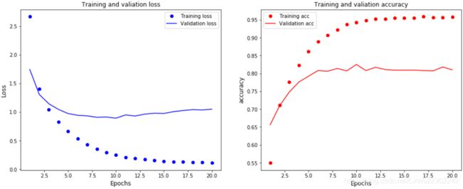
The network begins to overfit after ten epochs. Let’s train a new network from scratch for nine epochs and then evaluate it on the test set.
Retraining a model from scratch
model = keras.models.Sequential()
model.add( keras.layers.Dense(64, activation='relu', input_shape=(10000,)) ) #since 46 neurons
#you should avoid intermediate layers with many fewer than 46 hidden units(bottleneck).
model.add( keras.layers.Dense(64, activation='relu') )
model.add( keras.layers.Dense(46, activation='softmax') )

model.compile( optimizer='rmsprop', loss='categorical_crossentropy', metrics=['accuracy'] )
model.fit( x_train_partial, y_train_partial, epochs=10, batch_size=512, validation_data=(x_val, y_val) )
results = model.evaluate( x_test, one_hot_test_labels )

# Here are the final results:
results
This approach reaches an accuracy of ~80%. With a balanced binary classification problem, the accuracy reached by a purely random classifier would be 50%. But in this case it’s closer to 19% ( 0.18432769367764915 ), so the results seem pretty good, at least when compared to a random baseline:
import copy
import numpy as np

test_labels_copy = copy.copy(test_labels)
np.random.shuffle(test_labels_copy)
hits_array = np.array(test_labels) == np.array(test_labels_copy)
float(np.sum(hits_array)) / len(test_labels)![]()
Generating predictions for new data
You can verify that the predict method of the model instance returns a probability distribution over all 46 topics. Let’s generate topic predictions for all of the test data.
Generating predictions for new data
predictions = model.predict(x_test)Each entry in predictions is a vector of length 46:
predictions[0].shape![]()
The coefficients in this vector sum to 1:
np.sum(predictions[0])![]()
np.argmax(predictions[0])![]()
A different way to handle the labels and the loss
We mentioned earlier that another way to encode the labels would be to cast them as an integer tensor, like this:
y_train = np.array(train_labels)
y_test = np.array(test_labels)
The only thing this approach would change is the choice of the loss function. The loss function used in listing 3.21, categorical_crossentropy, expects the labels to follow a categorical encoding. With integer labels, you should use sparse_categorical_crossentropy:
This new loss function is still mathematically the same as categorical_crossentropy; it just has a different interface.
The importance of having sufficiently large intermediate layers
We mentioned earlier that because the final outputs are 46-dimensional, you should avoid intermediate layers with many fewer than 46 hidden units. Now let’s see what happens when you introduce an information bottleneck by having intermediate layers that are significantly less than 46-dimensional: for example, 4-dimensional.
A model with an information bottleneck
model = keras.models.Sequential()
model.add( keras.layers.Dense( 64, activation='relu', input_shape=(10000,)) )
model.add( keras.layers.Dense( 4, activation='relu') )
model.add( keras.layers.Dense(46, activation='softmax') )

model.compile( optimizer='rmsprop', loss='categorical_crossentropy', metrics=['accuracy'] )
model.fit(x_train_partial, y_train_partial, epochs=20, batch_size=128, validation_data=(x_val, y_val) )max( model.history.history['val_accuracy'] )![]()
The network now peaks at ~71% validation accuracy, an 8% absolute drop(results=[1.0128638812291866, 0.78762245]). This drop is mostly due to the fact that you’re trying to compress a lot of information (enough information to recover the separation hyperplanes of 46 classes) into an intermediate space that is too low-dimensional. The network is able to cram填满 most of the necessary information into these eight-dimensional representations, but not all of it.
Further experiments
- Try using larger or smaller layers: 32 units, 128 units, and so on.
- You used two hidden layers. Now try using a single hidden layer, or three hidden layers.
Wrapping up
Here’s what you should take away from this example:
- If you’re trying to classify data points among N classes, your network should end with a Dense layer of size N.
- In a single-label, multiclass classification problem, your network should end with a softmax activation so that it will output a probability distribution over the N output classes.
- Categorical crossentropy is almost always the loss function you should use for such problems. It minimizes the distance between the probability distributions output by the network and the true distribution of the targets.
- There are two ways to handle labels in multiclass classification:
– Encoding the labels via categorical encoding (also known as one-hot encoding) and using categorical_crossentropy as a loss function
– Encoding the labels as integers and using the sparse_categorical_crossentropy loss function
- If you need to classify data into a large number of categories, you should avoid creating information bottlenecks in your network due to intermediate layers that are too small.
Predicting house prices: a regression example
The two previous examples were considered classification problems, where the goal was to predict a single discrete label of an input data point. Another common type of machine-learning problem is regression, which consists of predicting a continuous value instead of a discrete label: for instance, predicting the temperature tomorrow, given meteorological[ˌmiːtiərəˈlɑːdʒɪkl]气象的 data; or predicting the time that a software project will take to
complete, given its specifications.
##########################
NOTE
Don’t confuse regression and the algorithm logistic regression. Confusingly, logistic regression isn’t a regression algorithm—it’s a classification algorithm.
##########################
The Boston Housing Price dataset
You’ll attempt to predict the median price of homes in a given Boston suburb in the mid-1970s, given data points about the suburb at the time, such as the crime rate, the local property tax rate, and so on. The dataset you’ll use has an interesting difference from the two previous examples. It has relatively few data points: only 506, split between 404 training samples and 102 test samples. And each feature in the input data (for example, the crime rate) has a different scale. For instance, some values are proportions, which take values between 0 and 1; others take values between 1 and 12, others between 0 and 100, and so on.
Loading the Boston housing dataset
from tensorflow.keras.datasets import boston_housing

(train_data, train_targets), (test_data, test_targets) = boston_housing.load_data()![]()
Let’s look at the data:
train_data.shape, test_data.shape((404, 13), (102, 13))As you can see, you have 404 training samples and 102 test samples, each with 13 numerical features, such as per capita crime rate, average number of rooms per dwelling寓所, accessibility to highways, and so on.
The targets are the median values of owner-occupied homes, in thousands of dollars:
train_targets[:5]![]()
max( train_targets ), min(train_targets) ![]()
The prices are typically between $5,000 and $50,000. If that sounds cheap, remember that this was the mid-1970s, and these prices aren’t adjusted for inflation.
Preparing the data
It would be problematic to feed into a neural network values that all take wildly different ranges. The network might be able to automatically adapt to such heterogeneous异质 data, but it would definitely make learning more difficult. A widespread best practice to deal with such data is to do feature-wise normalization: for each feature in the input data (a column in the input data matrix), you subtract the mean of the feature and divide by the standard deviation, so that the feature is centered around 0 and has a unit standard deviation. This is easily done in Numpy.
Normalizing the data
mean = train_data.mean( axis=0 )

train_data = train_data - mean
std = train_data.std(axis=0)
train_data = train_data/std

test_data = test_data - mean
test_data = test_data/std
Note that the quantities used for normalizing the test data are computed using the training data. You should never use in your workflow any quantity computed on the test data, even for something as simple as data normalization.
Building your network
Because so few samples are available, you’ll use a very small network with two hidden layers, each with 64 units. In general, the less training data you have, the worse overfitting will be, and using a small network is one way to mitigate overfitting.
Model definition
from tensorflow import keras
import tensorflow as tf
import numpy as np

def build_model():
    tf.random.set_seed(42)
    np.random.seed(42)
    model = keras.models.Sequential()                                #dimensions
    model.add( keras.layers.Dense(64, activation='relu', input_shape=(train_data.shape[1],))
             )
    model.add( keras.layers.Dense(64, activation='relu') )
    # scalar regression (a regression where you’re trying to predict a single continuous value)
    model.add( keras.layers.Dense(1) )

    model.compile( optimizer='rmsprop', loss='mse', metrics=['mae'] ) #Mean Absolute Error

    return model
The network ends with a single unit and no activation (it will be a linear layer). This is a typical setup for scalar regression (a regression where you’re trying to predict a single continuous value). Applying an activation function would constrain the range the output can take; for instance, if you applied a sigmoid activation function to the last layer, the network could only learn to predict values between 0 and 1. Here, because the last layer is purely linear, the network is free to learn to predict values in any range.
Note that you compile the network with the mse loss function—mean squared error, the square of the difference between the predictions and the targets. This is a widely used loss function for regression problems.
You’re also monitoring a new metric during training: mean absolute error (MAE). It’s the absolute value of the difference between the predictions and the targets. For instance, an MAE of 0.5 on this problem would mean your predictions are off by $500 on average(=0.5*1000).
Validating your approach using K-fold validation
To evaluate your network while you keep adjusting its parameters (such as the number of epochs used for training), you could split the data into a training set and a validation set, as you did in the previous examples. But because you have so few data points, the validation set would end up being very small (for instance, about 100 examples). As a consequence, the validation scores might change a lot depending on which data points you chose to use for validation and which you chose for training: the validation scores might have a high variance with regard to the validation split. This would prevent you from reliably evaluating your model.
The best practice in such situations is to use K-fold cross-validation (see figure 3.11). It consists of splitting the available data into K partitions (typically K = 4 or 5), instantiating实例化 K identical models, and training each one on K – 1 partitions while evaluating on the remaining partition. The validation score for the model used is then the average of the K validation scores obtained. In terms of code, this is straightforward.
Figure 3.11 3-fold cross-validation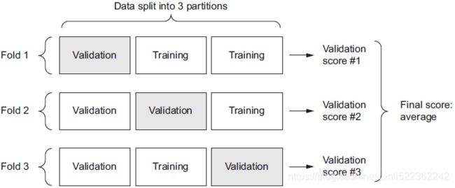
K-fold validation
k = 4
num_val_samples = len(train_data) // k
num_epochs = 100
all_scores = []

for i in range(k):
    print( 'processing fold #', i )
    val_data = train_data[ i*num_val_samples : (i+1)*num_val_samples ] ###
    val_targets = train_targets[ i* num_val_samples : (i+1)*num_val_samples ]

    train_data_partial = np.concatenate(
        [ train_data[:i*num_val_samples], train_data[(i+1)*num_val_samples:] ],
        axis=0
    )

    train_targets_partial = np.concatenate(
        [ train_targets[:i*num_val_samples], train_targets[(i+1)*num_val_samples:] ],
        axis=0
    )

    model = build_model()
    model.fit(train_data_partial, train_targets_partial, epochs = num_epochs, batch_size=1,
              verbose=0) # verbose=0 : Train the model in silent mode
    val_mse, val_mae = model.evaluate( val_data, val_targets, verbose=0 )
    all_scores.append( val_mae )
Running this with num_epochs = 100 yields the following results:
all_scores![]()
np.mean(all_scores)![]()
The different runs do indeed show rather different validation scores, from 2.2 to 2.7. The average (2.5) is a much more reliable metric than any single score—that’s the entire point of K-fold cross-validation. In this case, you’re off by $2,500 on average, which is significant considering that the prices range from $5,000 to $50,000.
Let’s try training the network a bit longer: 500 epochs. To keep a record of how well the model does at each epoch, you’ll modify the training loop to save the per epoch validation score log.
Saving the validation logs at each fold
k = 4
num_val_samples = len(train_data) // k
num_epochs = 500        ###
all_mae_histories = []  ###

for i in range(k):
    print('processing fold #', i)
    val_data = train_data[ i*num_val_samples: (i+1)*num_val_samples ]
    val_targets = train_targets[ i*num_val_samples: (i+1)*num_val_samples ]

    train_data_partial = np.concatenate(
        [ train_data[:i*num_val_samples], train_data[(i+1)*num_val_samples:]
        ], axis=0
    )

    train_targets_partial = np.concatenate(
        [ train_targets[:i*num_val_samples], train_targets[(i+1)*num_val_samples:]
        ], axis=0
    )

    model = build_model()

    history=model.fit(train_data_partial, train_targets_partial,
                      validation_data=(val_data, val_targets),
                      epochs=num_epochs, batch_size=1,
                      verbose=0) #Trains the model(in silent mode, verbose=0)
    mae_history = history.history['val_mae'] # 5000 epochs for fold i
    all_mae_histories.append(mae_history) # shape(k fold, epochs)
You can then compute the average of the per-epoch MAE scores for all folds
Building the history of successive mean K-fold validation scores
average_mae_history = [ np.mean([x[i] for x in all_mae_histories]) for i in range(num_epochs) ]Plotting validation scores
import matplotlib.pyplot as plt

plt.plot(range(1, len(average_mae_history)+1), average_mae_history)
plt.xlabel('Epochs')
plt.ylabel('Validation MAE')
plt.show()![]()
It may be a little difficult to see the plot, due to scaling issues(Larger range of vertical axis) and relatively high variance.
Let’s do the following:
- Omit the first 10 data points, which are on a different scale than the rest of the curve.
- Replace each point with an exponential moving average of the previous points, to obtain a smooth curve.
Plotting validation scores, excluding the first 10 data points
def smooth_curve(points, factor=0.81):
    smoothed_points = []
    for point in points:
        if smoothed_points:
            previous = smoothed_points[-1]#get the smoothed_point

            # exponentially weighted moving average chart(EWMA chart)
            # EMA = point*w + previous_EMA *(1-w) and w=2/(Number of days in EMA + 1)
            # for stock price:
            # EMA[position,period] =w* ClosePrice[position] + (100%-w) * EMA[position-1,period]
            # EMA[position,period] =(100%-w) * EMA[position-1,period] + w* ClosePrice[position]
            # EMA = previous_EMA *(1-w) + point*w and w=0.1(for this case)###################
            # ################# w=2/(10+1)=0.19 ==> factor =0.81
            # EMA = previous_EMA *0.81 + point*(1-0.81)
            smoothed_points.append( previous*factor + point*(1-factor))
        else:
            smoothed_points.append(point) #save first point
    return smoothed_points

smooth_mae_history = smooth_curve( average_mae_history[10:] )

plt.plot( range(1, len(smooth_mae_history)+1), smooth_mae_history )
plt.xlabel('Epochs')
plt.ylabel('Validation MAE')
plt.show()https://www.cnblogs.com/jiangxinyang/p/9705198.html
![]()
def smooth_curve(points, factor=0.9):
    smoothed_points = []
    for point in points:
        if smoothed_points:
            previous = smoothed_points[-1]#get the smoothed_point

            # exponentially weighted moving average chart(EWMA chart)
            # EMA = point*w + previous_EMA *(1-w) and w=2/(Number of days in EMA + 1)
            # for stock price:
            # EMA[position,period] =w* ClosePrice[position] + (100%-w) * EMA[position-1,period]
            # EMA[position,period] =(100%-w) * EMA[position-1,period] + w* ClosePrice[position]
            # EMA = previous_EMA *(1-w) + point*w and w=0.1(for this case)###################
            # ################# w=2/(10+1)=0.19 ==> factor =0.81
            # EMA = previous_EMA *0.81 + point*(1-0.81)
            smoothed_points.append( previous*factor + point*(1-factor))
        else:
            smoothed_points.append(point) #save first point
    return smoothed_points

smooth_mae_history = smooth_curve( average_mae_history[10:] )

plt.plot( range(1, len(smooth_mae_history)+1), smooth_mae_history )
plt.xlabel('Epochs')
plt.ylabel('Validation MAE')
plt.show()
np.argmin(smooth_mae_history) ![]()
According to this plot, validation MAE stops improving significantly after 36 epochs. Past that point, you start overfitting.
Once you’re finished tuning other parameters of the model (in addition to the number of epochs, you could also adjust the size of the hidden layers), you can train a final production model on all of the training data, with the best parameters, and then look at its performance on the test data.
model = build_model()
model.fit( train_data, train_targets, epochs=36, batch_size=16, verbose=0)
test_mse_score, test_mae_score = model.evaluate(test_data, test_targets)
test_mae_score
However, I found the test_mae_score > np.mean(all_scores) when num_epochs=100
model = build_model()
model.fit( train_data, train_targets, epochs=100, batch_size=16, verbose=0)
test_mse_score, test_mae_score = model.evaluate(test_data, test_targets)
test_mae_score
import pandas as pd
pd.DataFrame(average_mae_history).ewm(span=10, adjust=False, axis=0).mean().plot()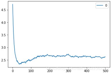
You’re still off by about $2,595
Wrapping up
Here’s what you should take away from this example:
- Regression is done using different loss functions than what we used for classification. Mean squared error (MSE) is a loss function commonly used for regression.
- Similarly, evaluation metrics to be used for regression differ from those used for classification; naturally, the concept of accuracy doesn’t apply for regression. A common regression metric is mean absolute error (MAE).
- When features in the input data have values in different ranges, each feature should be scaled independently as a preprocessing step.
- When there is little data available, using K-fold validation is a great way to reliably evaluate a model.
- When little training data is available, it’s preferable to use a small network with few hidden layers (typically only one or two), in order to avoid severe overfitting.
summary
- You’re now able to handle the most common kinds of machine-learning tasks on vector data: binary classification, multiclass classification, and scalar regression. The “Wrapping up” sections earlier in the chapter summarize the important points you’ve learned regarding these types of tasks.
- You’ll usually need to preprocess raw data before feeding it into a neural network.
- When your data has features with different ranges, scale each feature independently as part of preprocessing.
- As training progresses, neural networks eventually begin to overfit and obtain worse results on never-before-seen data.
- If you don’t have much training data, use a small network with only one or two hidden layers, to avoid severe overfitting.
- If your data is divided into many categories, you may cause information bottlenecks if you make the intermediate layers too small.
- Regression uses different loss functions and different evaluation metrics than classification.
- When you’re working with little data, K-fold validation can help reliably evaluate your model.
