【机器学习的学习笔记】（持续更新）

Notes of studying Machine Learning

Data Preprocessing

机器学习的学习笔记。

Supervised Learning

Supervised learning is the types of machine learning in which machines are trained using well “labelled” training data, and on basis of that data, machines predict the output. The labelled data means some input data is already tagged with the correct output.

In the real-world, supervised learning can be used for Risk Assessment, Image Classification, Fraud Detection, Spam Filtering, etc.

---

Regression

• a relationship between the input variable and the output variable
• the prediction of continuous variables, such as Weather Forecasting, Market Trends, etc.

Terminologies

• Dependent Variable: The main factor in Regression analysis which we want to predict or understand is called the dependent variable. It is also called target variable.

• Independent Variable: The factors which affect the dependent variables or which are used to predict the values of the dependent variables are called independent variable, also called as a predictor.

• Outliers: Outlier is an observation which contains either very low value or very high value in comparison to other observed values. An outlier may hamper the result, so it should be avoided.

• Multicollinearity: If the independent variables are highly correlated with each other than other variables, then such condition is called Multicollinearity. It should not be present in the dataset, because it creates problem while ranking the most affecting variable.

• Underfitting and Overfitting: If our algorithm works well with the training dataset but not well with test dataset, then such problem is called Overfitting. And if our algorithm does not perform well even with training dataset, then such problem is called underfitting.

---

Linear Regression

Simple Linear Regression

The key point in Simple Linear Regression is that the dependent variable must be a continuous/real value. However, the independent variable can be measured on continuous or categorical values.

A single Independent/Predictor(x) variable is used to model the response variable (Y)

$$Y=b_0+b_{1}x$$
Y = dependent variables (target variables),
X = Independent variables (predictor variables),
a and b are the linear coefficients

Steps:
Data Pre-processing Steps
Fitting the MLR model to the training set
Predicting the result of the test set

Multiple Linear Regression

More than one predictor variable to predict the response variable

$$Y=b_0+b_{1}x+b_{2}x+b_{3}x+.....+b_{n}x$$

import dataset

import pandas as pd
import numpy as npdf = pd.read_csv('/Users/haleyk/Documents/Python_Libraries_for_ML/Python_Libraries_for_ML/Supervised Learning/Linear Regression/homeprices.csv.xls')

area	bedrooms	age	price
0	2600	3.0	20	550000
1	3000	4.0	15	565000
2	3200	NaN	18	610000
3	3600	3.0	30	595000
4	4000	5.0	8	760000
5	4100	6.0	8	810000

remove NA

import math
median_bedrooms = math.floor(df.bedrooms.median())
median_bedrooms

df.bedrooms = df.bedrooms.fillna(median_bedrooms) # clean your data, Data Preprocessing: Fill NA values with median value of a column
df

	area	bedrooms	age	price
0	2600	3.0	20	550000
1	3000	4.0	15	565000
2	3200	4.0	18	610000
3	3600	3.0	30	595000
4	4000	5.0	8	760000
5	4100	6.0	8	810000

import model to find the relationship between area, bedrooms, age, and the price

from sklearn import linear_model
reg = linear_model.LinearRegression()
reg.fit(df[['area','bedrooms','age']],df.price)

"\nfrom sklearn.linear_model import LinearRegression\nreg = LinearRegression()\nreg.fit(df[['area','bedrooms','age']], df.price)\n"

this is a 2D array of shape (n_targets, n_features),
see how different factor change the price

reg.coef_
reg.intercept_
reg.predict([[3000,3,40]]) # 3000	4.0	15	565000 Find price of home with 3000 sqr ft area, 3 bedrooms, 40 year old

# return
array([498408.25158031])

reg.predict([[2500,4,5]]) # 2600	3.0	20	550000 Find price of home with 2500 sqr ft area, 4 bedrooms, 5 year old

# return
array([578876.03748933])

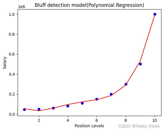
Polynomial Regression

Data points are arranged in a non-linear fashion, we need the Polynomial Regression model

$$Y=b_0+b_{1}x+b_2{x}^2+b_3{x}^3+.....+b_n{x}^n$$
Y is the predicted/target output, b0, b1,… bn are the regression coefficients. x is our independent/input variable.

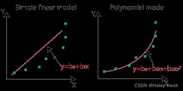
Photo Source

Steps:

1. Data Pre-processing

#importing libraries  
import numpy as np
import matplotlib.pyplot as plt 
import pandas as pd  
  
#importing datasets  
df = pd.read_csv('/Users/haleyk/Documents/Python_Libraries_for_ML/Python_Libraries_for_ML/Supervised Learning/Linear Regression/Position_Salaries.csv')
df

# return

Position	Level	Salary
0	Business Analyst	1	45000
1	Junior Consultant	2	50000
2	Senior Consultant	3	60000
3	Manager	4	80000
4	Country Manager	5	110000
5	Region Manager	6	150000
6	Partner	7	200000
7	Senior Partner	8	300000
8	C-level	9	500000
9	CEO	10	1000000

#Extracting Independent and dependent Variable  
X = df.iloc[:, 1:2].values  # level
y = df.iloc[:, 2].values  # salary

2. Build a Linear Regression model and fit it to the dataset

#Fitting the Linear Regression to the dataset  
from sklearn.linear_model import LinearRegression  
lin_regs= LinearRegression()  
lin_regs.fit(X,y)  

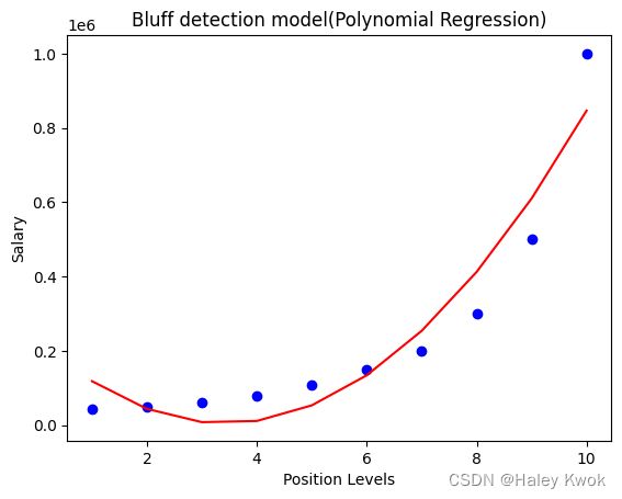
3. Build a Polynomial Regression model and fit it to the dataset

#Fitting the Polynomial regression to the dataset  
from sklearn.preprocessing import PolynomialFeatures  
poly_regs= PolynomialFeatures(degree= 2)  # the polynomial degree depends on our choice
x_poly= poly_regs.fit_transform(X)  # converting our feature matrix into polynomial feature matrix
lin_reg_2 =LinearRegression()  
lin_reg_2.fit(x_poly, y)  

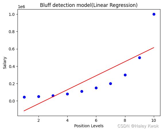
4. Visualize the result for Linear Regression and Polynomial Regression model

#Visulaizing the result for Linear Regression model  
plt.scatter(X,y,color="blue")  
plt.plot(X,lin_regs.predict(X), color="red")  
plt.title("Bluff detection model(Linear Regression)")  
plt.xlabel("Position Levels")  
plt.ylabel("Salary")  
plt.show()  

#Visulaizing the result for Polynomial Regression  
plt.scatter(X,y,color="blue")  
plt.plot(X, lin_reg_2.predict(poly_regs.fit_transform(X)), color="red")
plt.title("Bluff detection model(Polynomial Regression)")  
plt.xlabel("Position Levels")  
plt.ylabel("Salary")  
plt.show()  

#Fitting the Polynomial regression to the dataset by degree=3
from sklearn.preprocessing import PolynomialFeatures  
poly_regs= PolynomialFeatures(degree= 3)  # the polynomial degree depends on our choice
x_poly= poly_regs.fit_transform(X)  # converting our feature matrix into polynomial feature matrix
lin_reg_2 =LinearRegression()  
lin_reg_2.fit(x_poly, y)  

#Visulaizing the result for Polynomial Regression  
plt.scatter(X,y,color="blue")  
plt.plot(X, lin_reg_2.predict(poly_regs.fit_transform(X)), color="red")
plt.title("Bluff detection model(Polynomial Regression)")  
plt.xlabel("Position Levels")  
plt.ylabel("Salary")  
plt.show()  

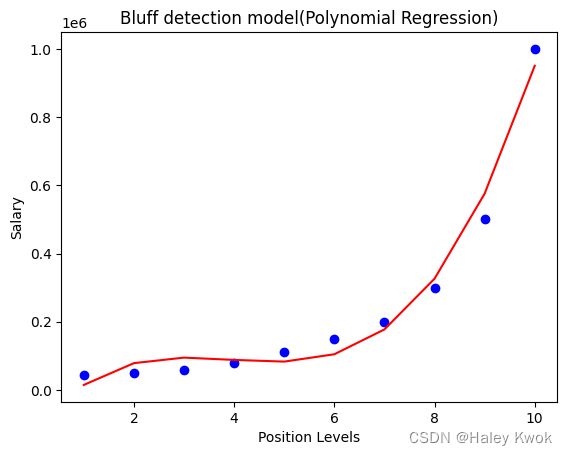
when degree=4, the curve is smoother and more accurate

5. Predicting the output

#Predicting the final result with the Linear Regression model:
lin_pred = lin_regs.predict([[6.5]])  
print(lin_pred)  

# return
[330378.78787879]

#Predicting the final result with the Polynomial Regression model:
poly_pred = lin_reg_2.predict(poly_regs.fit_transform([[6.5]]))  
print(poly_pred)  

# return
[158862.45265158]

Support Vector Regression

Decision Trees Regression

---

Classification

• the output variable is categorical

Binary Classifier

If the classification problem has only two possible outcomes, then it is called as Binary Classifier.
Examples: Yes-No, Male-Female, True-false, etc.

Multi-class Classifier

If a classification problem has more than two outcomes, then it is called as Multi-class Classifier.
Example: Classifications of types of crops, Classification of types of music.

Learners in Classification Problems

Lazy Learners

Lazy Learner firstly stores the training dataset and wait until it receives the test dataset. In Lazy learner case, classification is done on the basis of the most related data stored in the training dataset. It takes less time in training but more time for predictions.
Example: K-NN algorithm, Case-based reasoning

Eager Learners

Eager Learners develop a classification model based on a training dataset before receiving a test dataset. Opposite to Lazy learners, Eager Learner takes more time in learning, and less time in prediction.
Example: Decision Trees, Naïve Bayes, ANN.

Evaluating a Classification model

1. Log Loss or Cross-Entropy Loss

It is used for evaluating the performance of a classifier, whose output is a probability value between the 0 and 1.

For a good binary Classification model, the value of log loss should be near to 0.

2. Confusion Matrix

• True Negative: Model has given prediction No, and the real or actual value was also No.
• True Positive: The model has predicted yes, and the actual value was also true.
• False Negative: The model has predicted no, but the actual value was Yes, it is also called as Type-II error.
• False Positive: The model has predicted Yes, but the actual value was No. It is also called a Type-I error.

y_predicted = model.predict(X_test)
from sklearn.metrics import confusion matrix
cm = confusion_matrix(y_test, y_predicted)
import seaborn as sn
plt.figure(figsize = (10,7))
sn.heatmap(cm, annot = True)

3. AUC-ROC curve

ROC curve stands for Receiver Operating Characteristics Curve and AUC stands for Area Under the Curve.

The ROC curve is plotted with TPR and FPR, where TPR (True Positive Rate) on Y-axis and FPR(False Positive Rate) on X-axis.

---

Linear Model

Logistic Regression

$$f(x)=\frac{1}{1+e^{-x}}$$
uses sigmoid function or logistic function which is a complex cost function
f(x)= Output between the 0 and 1 value.
x= input to the function
e= base of natural logarithm.

Logistic Function (Sigmoid Function)
In logistic regression, we use the concept of the threshold value, which defines the probability of either 0 or 1. Such as values above the threshold value tends to 1, and a value below the threshold values tends to 0.

Assumptions
The dependent variable must be categorical in nature.
The independent variable should not have multi-collinearity.

Binomial

In binomial Logistic regression, there can be only two possible types of the dependent variables, such as 0 or 1, Pass or Fail, etc.

Steps:

1. Data Pre-processing step

#Data Pre-procesing Step  
# importing libraries  
import numpy as np
import matplotlib.pyplot as plt
import pandas as pd  
  
#importing datasets  
data_set= pd.read_csv('/Users/haleyk/Documents/Python_Libraries_for_ML/Python_Libraries_for_ML/Supervised Learning/Classification/Logistics Regression/User_Data.csv')  

#Extracting Independent and dependent Variable  
x= data_set.iloc[:, [2,3]].values  
y= data_set.iloc[:, 4].values  

# Splitting the dataset into training and test set.  
from sklearn.model_selection import train_test_split  
x_train, x_test, y_train, y_test= train_test_split(x, y, test_size= 0.25, random_state=0)  

#feature Scaling  
from sklearn.preprocessing import StandardScaler    
st_x= StandardScaler()    
x_train= st_x.fit_transform(x_train)    
x_test= st_x.transform(x_test)

# return
User ID	Gender	Age	EstimatedSalary	Purchased
0	15624510	Male	19	19000	0
1	15810944	Male	35	20000	0
2	15668575	Female	26	43000	0
3	15603246	Female	27	57000	0
4	15804002	Male	19	76000	0
...	...	...	...	...	...
395	15691863	Female	46	41000	1
396	15706071	Male	51	23000	1
397	15654296	Female	50	20000	1
398	15755018	Male	36	33000	0
399	15594041	Female	49	36000	1
400 rows × 5 columns

2. Fitting Logistic Regression to the Training set

#Fitting Logistic Regression to the training set  
from sklearn.linear_model import LogisticRegression  
classifier= LogisticRegression(random_state=0)  
classifier.fit(x_train, y_train)  

LogisticRegression(C=1.0, class_weight=None, dual=False, fit_intercept=True,  
                   intercept_scaling=1, l1_ratio=None, max_iter=100,  
                   multi_class='warn', n_jobs=None, penalty='l2',  
                   random_state=0, solver='warn', tol=0.0001, verbose=0,  
                   warm_start=False)  

3. Predicting the test result

#Predicting the test set result  
y_pred= classifier.predict(x_test)  

4. Test accuracy of the result(Creation of Confusion matrix)

#Creating the Confusion matrix  
from sklearn.metrics import confusion_matrix  
cm= confusion_matrix(y_test, y_pred)  

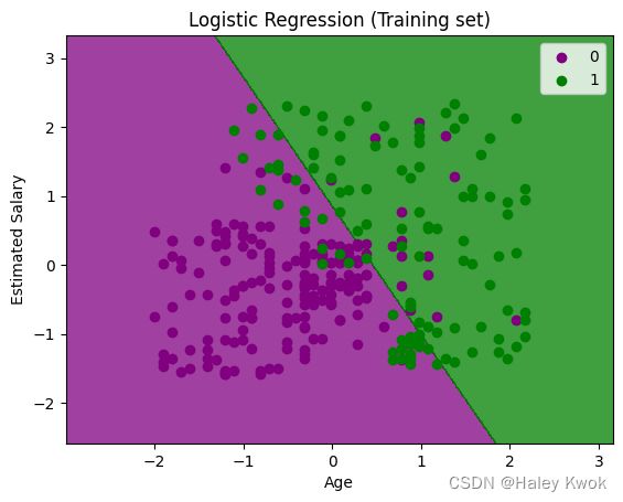
5. Visualizing the test set result

#Visualizing the training set result  
from matplotlib.colors import ListedColormap  
x_set, y_set = x_train, y_train  
x1, x2 = np.meshgrid(np.arange(start = x_set[:, 0].min() - 1, stop = x_set[:, 0].max() + 1, step  =0.01),  
np.arange(start = x_set[:, 1].min() - 1, stop = x_set[:, 1].max() + 1, step = 0.01))  
plt.contourf(x1, x2, classifier.predict(np.array([x1.ravel(), x2.ravel()]).T).reshape(x1.shape),  
alpha = 0.75, cmap = ListedColormap(('purple','green' )))  
plt.xlim(x1.min(), x1.max())  
plt.ylim(x2.min(), x2.max())  
for i, j in enumerate(np.unique(y_set)):  
    plt.scatter(x_set[y_set == j, 0], x_set[y_set == j, 1],  
        c = ListedColormap(('purple', 'green'))(i), label = j)  
plt.title('Logistic Regression (Training set)')  
plt.xlabel('Age')  
plt.ylabel('Estimated Salary')  
plt.legend()  
plt.show()  

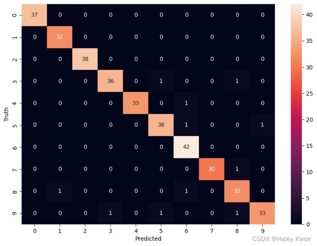
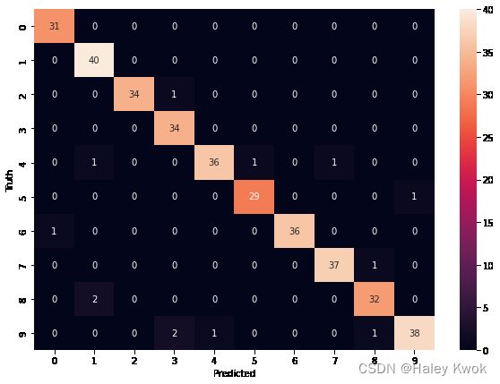
Multinomial

In multinomial Logistic regression, there can be 3 or more possible unordered types of the dependent variable, such as “cat”, “dogs”, or “sheep”

from sklearn.datasets import load_digits
%matplotlib inline
import matplotlib.pyplot as plt
digits = load_digits()

dir(digits)

digits.data[0] #number 0

from sklearn.linear_model import LogisticRegression
model = LogisticRegression()

from sklearn.model_selection import train_test_split

X_train, X_test, y_train, y_test = train_test_split(digits.data,digits.target, test_size=0.2)

model.fit(X_train, y_train)

model.score(X_test, y_test)

# return
0.9694444444444444

y_predicted = model.predict(X_test)
from sklearn.metrics import confusion_matrix
cm = confusion_matrix(y_test, y_predicted)
cm

import seaborn as sn
plt.figure(figsize = (10,7))
sn.heatmap(cm, annot=True)
plt.xlabel('Predicted')
plt.ylabel('Truth')

Ordinal

In ordinal Logistic regression, there can be 3 or more possible ordered types of dependent variables, such as “low”, “Medium”, or “High”.

---

Non-linear Model

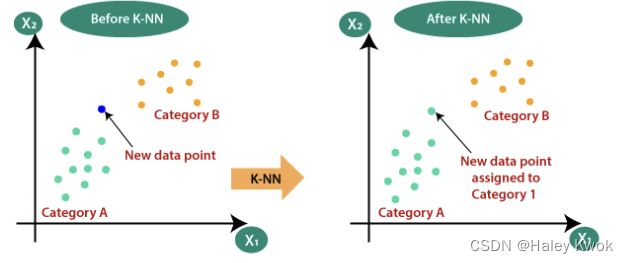
Lazy Learners: K-Nearest Neighbours

K-NN is a non-parametric algorithm, which means it does not make any assumption on underlying data.
KNN algorithm at the training phase just stores the dataset and when it gets new data, then it classifies that data into a category that is much similar to the new data.

Step-1: Select the number K of the neighbors
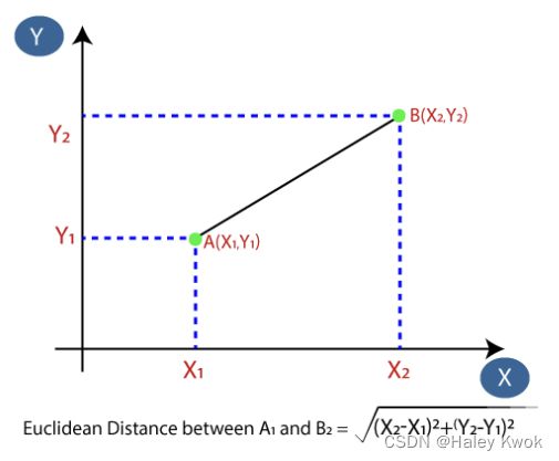
Step-2: Calculate the Euclidean distance of K number of neighbors
Step-3: Take the K nearest neighbors as per the calculated Euclidean distance.
Step-4: Among these k neighbors, count the number of the data points in each category.
Step-5: Assign the new data points to that category for which the number of the neighbor is maximum.
Step-6: Our model is ready.

1. Data Pre-processing step

import pandas as pd
from sklearn.datasets import load_iris
iris = load_iris()

iris.feature_names
# return
['sepal length (cm)',
 'sepal width (cm)',
 'petal length (cm)',
 'petal width (cm)']
 
iris.target_names
# return
array(['setosa', 'versicolor', 'virginica'], dtype=')

df = pd.DataFrame(iris.data,columns=iris.feature_names)
df.head()
# return
	sepal length (cm)	sepal width (cm)	petal length (cm)	petal width (cm)
0	5.1	3.5	1.4	0.2
1	4.9	3.0	1.4	0.2
2	4.7	3.2	1.3	0.2
3	4.6	3.1	1.5	0.2
4	5.0	3.6	1.4	0.2

df['target']=iris.target
df.head()
# return

sepal length (cm)	sepal width (cm)	petal length (cm)	petal width (cm)	target
0	5.1	3.5	1.4	0.2	0
1	4.9	3.0	1.4	0.2	0
2	4.7	3.2	1.3	0.2	0
3	4.6	3.1	1.5	0.2	0
4	5.0	3.6	1.4	0.2	0

df['flower_name'] =df.target.apply(lambda x: iris.target_names[x])
df.head()
# return
sepal length (cm)	sepal width (cm)	petal length (cm)	petal width (cm)	target	flower_name
0	5.1	3.5	1.4	0.2	0	setosa
1	4.9	3.0	1.4	0.2	0	setosa
2	4.7	3.2	1.3	0.2	0	setosa
3	4.6	3.1	1.5	0.2	0	setosa
4	5.0	3.6	1.4	0.2	0	setosa

2. Fitting the K-NN algorithm to the Training set

from sklearn.model_selection import train_test_split

X = df.drop(['target','flower_name'], axis='columns')
y = df.target

from sklearn.neighbors import KNeighborsClassifier
knn = KNeighborsClassifier(n_neighbors=10) # Number of neighbors to use by default for 

knn.fit(X_train, y_train)
# return
KNeighborsClassifier(n_neighbors=10)

knn.fit(X_test, y_test)
# return
KNeighborsClassifier(n_neighbors=10)

3. Predicting the test result

knn.predict([[4.8,3.0,1.5,0.3]])
# return
/Users/haleyk/opt/anaconda3/lib/python3.8/site-packages/sklearn/base.py:450: UserWarning: X does not have valid feature names, but KNeighborsClassifier was fitted with feature names
  warnings.warn(
array([0])

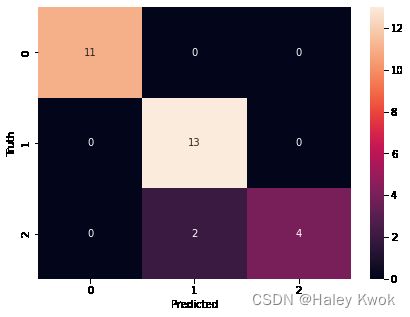
4. Test accuracy of the result(Creation of Confusion matrix)

from sklearn.metrics import confusion_matrix
y_pred = knn.predict(X_test)
cm = confusion_matrix(y_test, y_pred)
cm

# return
array([[11,  0,  0],
       [ 0, 13,  0],
       [ 0,  2,  4]])

%matplotlib inline
import matplotlib.pyplot as plt
import seaborn as sn
plt.figure(figsize=(7,5))
sn.heatmap(cm, annot=True)
plt.xlabel('Predicted')
plt.ylabel('Truth')

# 11+13+2+4 = 30 test set
# 2 is wrong
# there is only 2 wrong, therefore, the score is 0.933333

knn.score(X_test, y_test)
# return
0.9333333333333333

5. Print classification report for precision, recall and f1-score for each classes

from sklearn.metrics import classification_report

print(classification_report(y_test, y_pred))

# return
    precision    recall  f1-score   support

           0       1.00      1.00      1.00        11
           1       0.87      1.00      0.93        13
           2       1.00      0.67      0.80         6

    accuracy                           0.93        30
   macro avg       0.96      0.89      0.91        30
weighted avg       0.94      0.93      0.93        30

1. Data Pre-processing step

# importing libraries  
import numpy as np  
import matplotlib.pyplot as plt  
import pandas as pd  
  
#importing datasets  
data_set= pd.read_csv('/Users/haleyk/Documents/Python_Libraries_for_ML/Python_Libraries_for_ML/Supervised Learning/Classification/Logistics Regression/User_Data.csv')  
data_set

User ID	Gender	Age	EstimatedSalary	Purchased
0	15624510	Male	19	19000	0
1	15810944	Male	35	20000	0
2	15668575	Female	26	43000	0
3	15603246	Female	27	57000	0
4	15804002	Male	19	76000	0
...	...	...	...	...	...
395	15691863	Female	46	41000	1
396	15706071	Male	51	23000	1
397	15654296	Female	50	20000	1
398	15755018	Male	36	33000	0
399	15594041	Female	49	36000	1
400 rows × 5 columns

2. Fitting the K-NN algorithm to the Training set

#Extracting Independent and dependent Variable  
x= data_set.iloc[:, [2,3]].values  
y= data_set.iloc[:, 4].values  
  
# Splitting the dataset into training and test set.  
from sklearn.model_selection import train_test_split  
x_train, x_test, y_train, y_test= train_test_split(x, y, test_size= 0.25, random_state=0)  
  
#feature Scaling  
from sklearn.preprocessing import StandardScaler    
st_x= StandardScaler()    
x_train= st_x.fit_transform(x_train)    
x_test= st_x.transform(x_test)  

#Fitting K-NN classifier to the training set  
from sklearn.neighbors import KNeighborsClassifier  
classifier= KNeighborsClassifier(n_neighbors=5, metric='minkowski', p=2 )  
classifier.fit(x_train, y_train)  

3. Predicting the test result

#Predicting the test set result  
y_pred= classifier.predict(x_test)  

4. Test accuracy of the result(Creation of Confusion matrix)

#Creating the Confusion matrix  
from sklearn.metrics import confusion_matrix  
cm= confusion_matrix(y_test, y_pred)  

5. Visualizing the test set result

#Visulaizing the training set result  
from matplotlib.colors import ListedColormap  
x_set, y_set = x_train, y_train  
x1, x2 = np.meshgrid(np.arange(start = x_set[:, 0].min() - 1, stop = x_set[:, 0].max() + 1, step  =0.01),  
np.arange(start = x_set[:, 1].min() - 1, stop = x_set[:, 1].max() + 1, step = 0.01))  
plt.contourf(x1, x2, classifier.predict(np.array([x1.ravel(), x2.ravel()]).T).reshape(x1.shape),  
alpha = 0.75, cmap = ListedColormap(('red','green' )))  
plt.xlim(x1.min(), x1.max())  
plt.ylim(x2.min(), x2.max())  
for i, j in enumerate(np.unique(y_set)):  
    plt.scatter(x_set[y_set == j, 0], x_set[y_set == j, 1],  
        c = ListedColormap(('red', 'green'))(i), label = j)  
plt.title('K-NN Algorithm (Training set)')  
plt.xlabel('Age')  
plt.ylabel('Estimated Salary')  
plt.legend()  
plt.show()  

#Visualizing the test set result  
from matplotlib.colors import ListedColormap  
x_set, y_set = x_test, y_test  
x1, x2 = np.meshgrid(np.arange(start = x_set[:, 0].min() - 1, stop = x_set[:, 0].max() + 1, step  =0.01),  
np.arange(start = x_set[:, 1].min() - 1, stop = x_set[:, 1].max() + 1, step = 0.01))  
plt.contourf(x1, x2, classifier.predict(np.array([x1.ravel(), x2.ravel()]).T).reshape(x1.shape),  
alpha = 0.75, cmap = ListedColormap(('red','green' )))  
plt.xlim(x1.min(), x1.max())  
plt.ylim(x2.min(), x2.max())  
for i, j in enumerate(np.unique(y_set)):  
    plt.scatter(x_set[y_set == j, 0], x_set[y_set == j, 1],  
        c = ListedColormap(('red', 'green'))(i), label = j)  
plt.title('K-NN algorithm(Test set)')  
plt.xlabel('Age')  
plt.ylabel('Estimated Salary')  
plt.legend()  
plt.show()  

Eager Learners: Decision Trees

• solve problems for both categorical and numerical data
• builds a tree-like structure in which each internal node represents the “test” for an attribute, each branch represent the result of the test, and each leaf node represents the final decision or result.
• is constructed starting from the root node/parent node (dataset), which splits into left and right child nodes (subsets of dataset). These child nodes are further divided into their children node, and themselves become the parent node of those nodes.

Terminologies

Root Node: Root node is from where the decision tree starts. It represents the entire dataset, which further gets divided into two or more homogeneous sets.

Leaf Node: Leaf nodes are the final output node, and the tree cannot be segregated further after getting a leaf node.

Splitting: Splitting is the process of dividing the decision node/root node into sub-nodes according to the given conditions.

Branch/Sub Tree: A tree formed by splitting the tree.

Pruning: Pruning is the process of removing the unwanted branches from the tree.

Parent/Child node: The root node of the tree is called the parent node, and other nodes are called the child nodes.

Step-1: Begin the tree with the root node, says S, which contains the complete dataset.
Step-2: Find the best attribute in the dataset using Attribute Selection Measure (ASM).

1. Information Gain
   Information gain is the measurement of changes in entropy after the segmentation of a dataset based on an attribute.

Information Gain= Entropy(S)- [(Weighted Avg) *Entropy(each feature)

Entropy: Entropy is a metric to measure the impurity in a given attribute. It specifies randomness in data. Entropy can be calculated as:

Entropy(s)= -P(yes)log2 P(yes)- P(no) log2 P(no)

2. Gini Index
   Gini index is a measure of impurity or purity used while creating a decision tree in the CART(Classification and Regression Tree) algorithm.

An attribute with the low Gini index should be preferred as compared to the high Gini index.

$$GiniIndex=1-\sum j_P{j}_2$$

Step-3: Divide the S into subsets that contains possible values for the best attributes.
Step-4: Generate the decision tree node, which contains the best attribute.
Step-5: Recursively make new decision trees using the subsets of the dataset created in step -3. Continue this process until a stage is reached where you cannot further classify the nodes and called the final node as a leaf node.

1. Data Pre-Processing Step

2. Fitting a Decision-Tree algorithm to the Training set

#Fitting Decision Tree classifier to the training set  
From sklearn.tree import DecisionTreeClassifier  
classifier= DecisionTreeClassifier(criterion='entropy', random_state=0)  
classifier.fit(x_train, y_train)  

"criterion=‘entropy’: Criterion is used to measure the quality of split, which is calculated by information gain given by entropy.

3. Predicting the test result

#Predicting the test set result  
y_pred= classifier.predict(x_test)  

4. Test accuracy of the result (Creation of Confusion matrix)

#Creating the Confusion matrix  
from sklearn.metrics import confusion_matrix  
cm= confusion_matrix(y_test, y_pred)  

# return
array([[62,  6],
       [ 3, 29]])

In the above output image, we can see the confusion matrix, which has 6+3= 9 incorrect predictions and 62+29=91 correct predictions. Therefore, we can say that compared to other classification models, the Decision Tree classifier made a good prediction.

Another example:

import pandas as pd
df = pd.read_csv('/Users/haleyk/Desktop/Codebasics/ML/9_decision_tree/Exercise/titanic.csv')
df.head()

df.drop(['PassengerId','Name','SibSp','Parch','Ticket','Cabin','Embarked'],axis=1,inplace=True)
df.head()

df.Sex = df.Sex.map({'female':1, 'male':0})  
df.Sex

df = df.fillna(df.Age.mean())
df

df.isnull().sum()

X = df.drop('Survived',axis='columns')
y = df.Survived

X
# return
	Pclass	Sex	Age	Fare
0	3	0	22.000000	7.2500
1	1	1	38.000000	71.2833
2	3	1	26.000000	7.9250
3	1	1	35.000000	53.1000
4	3	0	35.000000	8.0500
...	...	...	...	...
886	2	0	27.000000	13.0000
887	1	1	19.000000	30.0000
888	3	1	29.699118	23.4500
889	1	0	26.000000	30.0000
890	3	0	32.000000	7.7500
891 rows × 4 columns

y 
# return
0      0
1      1
2      1
3      1
4      0
      ..
886    0
887    1
888    0
889    1
890    0
Name: Survived, Length: 891, dtype: int64

from sklearn.model_selection import train_test_split
X_train, X_test, y_train, y_test = train_test_split(X,y, test_size=0.2)

from sklearn import tree
model = tree.DecisionTreeClassifier()
model.fit(X_train,y_train)
# return
DecisionTreeClassifier()

model.score(X_test,y_test)
# return
0.8044692737430168

Random Forest [Overfitting]

• is one of the most powerful supervised learning algorithms which is capable of performing regression as well as classification tasks.
• is an ensemble learning method which combines multiple decision trees and predicts the final output based on the average of each tree output. The combined decision trees are called as base models.
• uses Bagging or Bootstrap Aggregation technique of ensemble learning in which aggregated decision tree runs in parallel and do not interact with each other.

$$g(x)=f_0(x)+f_1(x)+f_2(x)+...$$

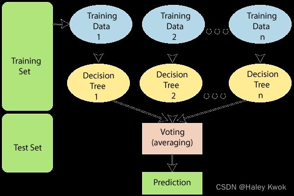
Photo Source

Step-1: Select random K data points from the training set.

Step-2: Build the decision trees associated with the selected data points (Subsets).

Step-3: Choose the number N for decision trees that you want to build.

Step-4: Repeat Step 1 & 2.

Step-5: For new data points, find the predictions of each decision tree, and assign the new data points to the category that wins the majority votes.

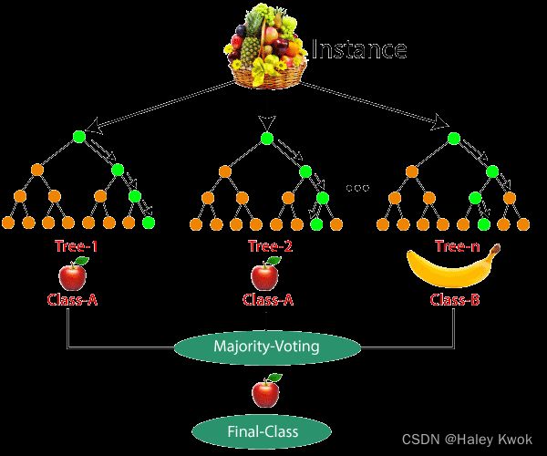
Photo Source

import pandas as pd
from sklearn.datasets import load_digits
digits = load_digits()

dir(digits)   # list of string

# return
['DESCR', 'data', 'feature_names', 'frame', 'images', 'target', 'target_names']

df[0:12]

X = df.drop('target',axis=1)
y = df.target

from sklearn.model_selection import train_test_split
X_train, X_test, y_train, y_test = train_test_split(X,y,test_size=0.2)

from sklearn.ensemble import RandomForestClassifier
model = RandomForestClassifier(n_estimators=20) #The number of trees in the forest.
model.fit(X_train, y_train) 

# return
RandomForestClassifier(n_estimators=20)

model.score(X_test, y_test)
# return
0.9638888888888889

from sklearn.metrics import confusion_matrix
cm = confusion_matrix(y_test, y_predicted)
cm

%matplotlib inline
import matplotlib.pyplot as plt
import seaborn as sn
plt.figure(figsize=(10,7))
sn.heatmap(cm, annot=True)
plt.xlabel('Predicted')
plt.ylabel('Truth')

# return
Text(69.0, 0.5, 'Truth')

---

Eager Learners: Naïve Bayes

Bernoulli, Multinomial and Gaussian Naive Bayes

• Multinomial Naïve Bayes consider a feature vector where a given term represents the number of times it appears or very often i.e. frequency.
• On the other hand, Bernoulli is a binary algorithm used when the feature is present or not.
• At last Gaussian is based on continuous distribution.

Naïve Bayes algorithm is a supervised learning algorithm, which is based on Bayes theorem and used for solving classification problems.

It is mainly used in text classification that includes a high-dimensional training dataset.

It is a probabilistic classifier, which means it predicts on the basis of the probability of an object.

Some popular examples of Naïve Bayes Algorithm are spam filtration, Sentimental analysis, and classifying articles.

• Naïve: It is called Naïve because it assumes that the occurrence of a certain feature is independent of the occurrence of other features. Such as if the fruit is identified on the bases of color, shape, and taste, then red, spherical, and sweet fruit is recognized as an apple. Hence each feature individually contributes to identify that it is an apple without depending on each other.
• Bayes: It is called Bayes because it depends on the principle of Bayes’ Theorem.

Bayes’ Theorem
P(A|B) = P(B|A)P(A) / P(B)

Assumption

Naive bayes theorm uses bayes theorm for conditional probability with a naive assumption that the features are not correlated to each other and tries to find conditional probability of target variable given the probabilities of features.

import pandas as pd
df = pd.read_csv('https://storage.googleapis.com/kagglesdsdata/competitions/3136/26502/train.csv?GoogleAccessId=web-data@kaggle-161607.iam.gserviceaccount.com&Expires=1646132661&Signature=PteVGgxccUCBs%2FsS7tCMNObj%2B6Svdf23ERl7SVnvVns2y4B7yPqW3mYYNQazGsbpEF6P0KUiKysl5ZTjIZEuNI%2FdduFeY77DWHdNVWZGDd5TlizWxOPd1E2rHcOyYpavsCr1OgtjLU8HpTCDsHhTb9kpzGoSK0Dzf2iFgh7HNWCsUYbHjCK9OAn6IBITg%2BZpn2KagdtPMFR3QWDeQV5kHlpsG9j8DaPdQGyJcZBC%2B8zuqz2UM6tknZp20fVDjtWR5ZvklfjzDpWGVtKxZfpFQlAv4f3udqF%2F%2F1j2zXFUcUXiD6tFdDR40rcNTL%2BVDJnUeNFHX4%2F7XbprMuToqMgpqQ%3D%3D&response-content-disposition=attachment%3B+filename%3Dtrain.csv')
df.head()

# return
PassengerId	Survived	Pclass	Name	Sex	Age	SibSp	Parch	Ticket	Fare	Cabin	Embarked
0	1	0	3	Braund, Mr. Owen Harris	male	22.0	1	0	A/5 21171	7.2500	NaN	S
1	2	1	1	Cumings, Mrs. John Bradley (Florence Briggs Th...	female	38.0	1	0	PC 17599	71.2833	C85	C
2	3	1	3	Heikkinen, Miss. Laina	female	26.0	0	0	STON/O2. 3101282	7.9250	NaN	S
3	4	1	1	Futrelle, Mrs. Jacques Heath (Lily May Peel)	female	35.0	1	0	113803	53.1000	C123	S
4	5	0	3	Allen, Mr. William Henry	male	35.0	0	0	373450	8.0500	NaN	S

df.drop(['PassengerId','Name','SibSp','Parch','Ticket','Cabin','Embarked'],axis='columns',inplace=True)
df.head()

# return
	Survived	Pclass	Sex	Age	Fare
0	0	3	male	22.0	7.2500
1	1	1	female	38.0	71.2833
2	1	3	female	26.0	7.9250
3	1	1	female	35.0	53.1000
4	0	3	male	35.0	8.0500

inputs = df.drop('Survived',axis='columns')
target = df.Survived

#inputs.Sex = inputs.Sex.map({'male': 1, 'female': 2})
dummies = pd.get_dummies(inputs.Sex)
dummies.head()

# return
	female	male
0	0	1
1	1	0
2	1	0
3	1	0
4	0	1

# merged

inputs = pd.concat([inputs,dummies],axis='columns')
inputs.head()

# return

Pclass	Sex	Age	Fare	female	male
0	3	male	22.0	7.2500	0	1
1	1	female	38.0	71.2833	1	0
2	3	female	26.0	7.9250	1	0
3	1	female	35.0	53.1000	1	0
4	3	male	35.0	8.0500	0	1

inputs.drop(['Sex','male'],axis='columns',inplace=True)
inputs.head()

# return

Pclass	Age	Fare	female
0	3	22.0	7.2500	0
1	1	38.0	71.2833	1
2	3	26.0	7.9250	1
3	1	35.0	53.1000	1
4	3	35.0	8.0500	0

inputs.columns[inputs.isna().any()] #detect missing data
# return
Index(['Age'], dtype='object')

inputs.Age[:10]
inputs.Age = inputs.Age.fillna(inputs.Age.mean()) # fill the NaN with mean value
inputs.head()

# return
	Pclass	Age	Fare	female
0	3	22.0	7.2500	0
1	1	38.0	71.2833	1
2	3	26.0	7.9250	1
3	1	35.0	53.1000	1
4	3	35.0	8.0500	0

from sklearn.model_selection import train_test_split
X_train, X_test, y_train, y_test = train_test_split(inputs,target,test_size=0.3)

from sklearn.naive_bayes import GaussianNB
model = GaussianNB()

len(X_train)
# 623
len(X_test)
# 268
len(inputs)
# 891

model.fit(X_train,y_train)
model.score(X_test,y_test)
# return
0.7350746268656716

# Calculate the score using cross validation
from sklearn.model_selection import cross_val_score
cross_val_score(GaussianNB(),X_train, y_train, cv=5)
# return
array([0.784     , 0.808     , 0.784     , 0.76612903, 0.82258065])

Support Vector Machines (SVM)

Support Vector Machine is a supervised learning algorithm which can be used for regression as well as classification problems. So if we use it for regression problems, then it is termed as Support Vector Regression.

Photo Source

Linear SVM

Linear SVM is used for linearly separable data, which means if a dataset can be classified into two classes by using a single straight line, then such data is termed as linearly separable data, and classifier is used called as Linear SVM classifier.

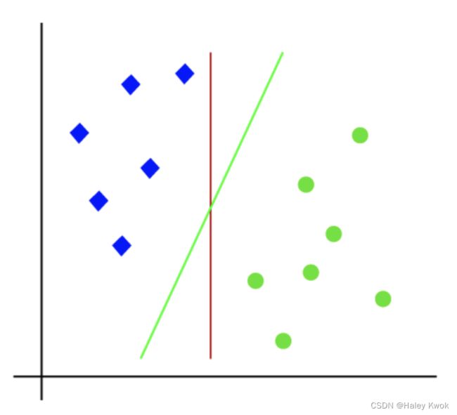
Photo Source

#Data Pre-processing Step  
# importing libraries  
import numpy as nm  
import matplotlib.pyplot as mtp  
import pandas as pd  
  
#importing datasets  
data_set= pd.read_csv('/Users/haleyk/Documents/Python_Libraries_for_ML/Python_Libraries_for_ML/Supervised Learning/Classification/Logistics Regression/User_Data.csv')  
data_set

# return

User ID	Gender	Age	EstimatedSalary	Purchased
0	15624510	Male	19	19000	0
1	15810944	Male	35	20000	0
2	15668575	Female	26	43000	0
3	15603246	Female	27	57000	0
4	15804002	Male	19	76000	0
...	...	...	...	...	...
395	15691863	Female	46	41000	1
396	15706071	Male	51	23000	1
397	15654296	Female	50	20000	1
398	15755018	Male	36	33000	0
399	15594041	Female	49	36000	1
400 rows × 5 columns

#Extracting Independent and dependent Variable  
x= data_set.iloc[:, [2,3]].values  
y= data_set.iloc[:, 4].values  
  
# Splitting the dataset into training and test set.  
from sklearn.model_selection import train_test_split  
x_train, x_test, y_train, y_test= train_test_split(x, y, test_size= 0.25, random_state=0)  
#feature Scaling  
from sklearn.preprocessing import StandardScaler    
st_x= StandardScaler()    
x_train= st_x.fit_transform(x_train)    
x_test= st_x.transform(x_test)     

from sklearn.svm import SVC # "Support vector classifier"  
classifier = SVC(kernel='linear', random_state=0)  
classifier.fit(x_train, y_train)  

#Predicting the test set result  
y_pred= classifier.predict(x_test)  

#Creating the Confusion matrix  
from sklearn.metrics import confusion_matrix  
cm= confusion_matrix(y_test, y_pred)  
cm

# return
array([[66,  2],
       [ 8, 24]])

import pandas as pd
from sklearn.datasets import load_iris
iris = load_iris()


df['flower_name'] =df.target.apply(lambda x: iris.target_names[x])
df.head()

df['target'] = iris.target  #0-49 setosa
df.head(

df[df.target==1].head() #50-99 versicolor

df[df.target==2].head() #100-149 virginica

df['flower_name'] =df.target.apply(lambda x: iris.target_names[x])
df.head()

from sklearn.model_selection import train_test_split
X = df.drop(['target','flower_name'], axis=1)
y = df.target

X_train, X_test, y_train, y_test = train_test_split(X, y, test_size=0.2)

from sklearn.svm import SVC
model = SVC()

model.fit(X_train, y_train)

model.score(X_test, y_test)

# return
model.predict([[4.8,3.0,1.5,0.3]])

Tune Parameter

# Regularization (C)
model_C = SVC(C=1)
model_C.fit(X_train, y_train)
model_C.score(X_test, y_test)


model_C = SVC(C=10)
model_C.fit(X_train, y_train)
model_C.score(X_test, y_test)


# Gamma
model_g = SVC(gamma=10)
model_g.fit(X_train, y_train)
model_g.score(X_test, y_test)

# Kernel 
model_linear_kernal = SVC(kernel='linear')
model_linear_kernal.fit(X_train, y_train)
model_linear_kernal.score(X_test, y_test)

Non-linear SVM (Kernel SVM)

Non-Linear SVM is used for non-linearly separated data, which means if a dataset cannot be classified by using a straight line, then such data is termed as non-linear data and classifier used is called as Non-linear SVM classifier.

Photo Source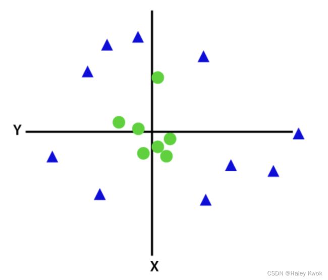

To separate these data points, we need to add one more dimension. For linear data, we have used two dimensions x and y, so for non-linear data, we will add a third dimension z.

$$z=x^2+y^2$$

#Data Pre-processing Step  
# importing libraries  
import numpy as nm  
import matplotlib.pyplot as mtp  
import pandas as pd  
  
#importing datasets  
data_set= pd.read_csv('user_data.csv')  
  
#Extracting Independent and dependent Variable  
x= data_set.iloc[:, [2,3]].values  
y= data_set.iloc[:, 4].values  
  
# Splitting the dataset into training and test set.  
from sklearn.model_selection import train_test_split  
x_train, x_test, y_train, y_test= train_test_split(x, y, test_size= 0.25, random_state=0)  
#feature Scaling  
from sklearn.preprocessing import StandardScaler    
st_x= StandardScaler()    
x_train= st_x.fit_transform(x_train)    
x_test= st_x.transform(x_test)  

---

Dimensionality Reduction

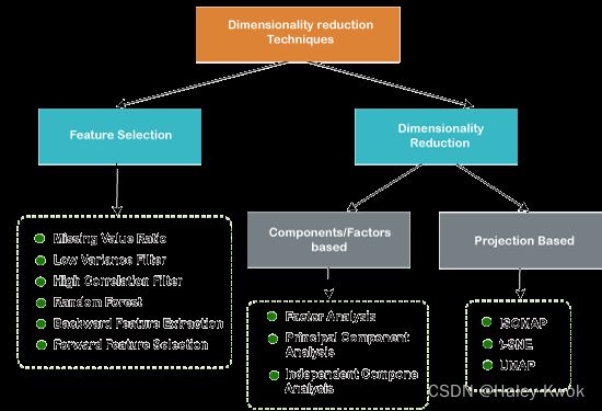
Photo Source

Filters Methods

In this method, the dataset is filtered, and a subset that contains only the relevant features is taken. Some common techniques of filters method are:

Correlation
Chi-Square Test
ANOVA
Information Gain, etc.

Wrappers Methods

The performance decides whether to add those features or remove to increase the accuracy of the model. This method is more accurate than the filtering method but complex to work. Some common techniques of wrapper methods are:

Forward Selection
Backward Selection
Bi-directional Elimination

Embedded Methods

Embedded methods check the different training iterations of the machine learning model and evaluate the importance of each feature. Some common techniques of Embedded methods are:

Elastic Net

Lasso Regression/ L1 regularization [Reduce complexity]

• penalty term contains only the absolute weights
• can only shrink the slope to 0 because of taking absolute values

$$Loss=Error(Y-Y)+\lambda \sum _1^n|w_i|$$

# import libraries
from sklearn.linear_model import Lasso
lasso_reg = Lasso(alpha=50, max_iter=100, tol=0.1)
lasso_reg.fit(train_X, train_y)

lasso_reg.score(test_X, test_y)
# return
0.6636
lasso_reg.score(train_X, train_y)
# return
0.6766

---

Ridge Regression/ L2 regularization [Reduce complexity]

• a general linear or polynomial regression will fail if there is high collinearity between the independent variables
• penalty term contains a square of weights
• shrink the slope near to 0

$$Loss=Error(Y-Y)+\lambda \sum _1^n{w}_i^2$$

from sklearn.linear_model import Ridge
ridge_reg= Ridge(alpha=50, max_iter=100, tol=0.1)
ridge_reg.fit(train_X, train_y)

ridge_reg.score(test_X, test_y)
# return
0.6670848945194956

ridge_reg.score(train_X, train_y)
# return
0.6622376739684328

Feature Extractions

Principal Component Analysis (Unsupervised Learning)

Principal Component Analysis is a statistical process that converts the observations of correlated features into a set of linearly uncorrelated features with the help of orthogonal transformation. These new transformed features are called the Principal Components. It is one of the popular tools that is used for exploratory data analysis and predictive modeling.

from sklearn.decomposition import PCA

pca = PCA(0.95)
X_pca = pca.fit_transform(X)
X_pca.shape

# return
(1797, 29)

pca.explained_variance_ratio_
# return
array([0.14890594, 0.13618771, 0.11794594, 0.08409979, 0.05782415,
       0.0491691 , 0.04315987, 0.03661373, 0.03353248, 0.03078806,
       0.02372341, 0.02272697, 0.01821863, 0.01773855, 0.01467101,
       0.01409716, 0.01318589, 0.01248138, 0.01017718, 0.00905617,
       0.00889538, 0.00797123, 0.00767493, 0.00722904, 0.00695889,
       0.00596081, 0.00575615, 0.00515158, 0.0048954 ])

pca.n_components_
# return
29

X_pca
# return
array([[ -1.25946645,  21.27488348,  -9.46305462, ...,   3.67072108,
         -0.9436689 ,  -1.13250195],
       [  7.9576113 , -20.76869896,   4.43950604, ...,   2.18261819,
         -0.51022719,   2.31354911],
       [  6.99192297,  -9.95598641,   2.95855808, ...,   4.22882114,
          2.1576573 ,   0.8379578 ],
       ...,
       [ 10.8012837 ,  -6.96025223,   5.59955453, ...,  -3.56866194,
          1.82444444,   3.53885886],
       [ -4.87210009,  12.42395362, -10.17086635, ...,   3.25330054,
          0.95484174,  -0.93895602],
       [ -0.34438963,   6.36554919,  10.77370849, ...,  -3.01636722,
          1.29752723,   2.58810313]])

X_train_pca, X_test_pca, y_train, y_test = train_test_split(X_pca, y, test_size=0.2, random_state=30)

from sklearn.linear_model import LogisticRegression
model = LogisticRegression(max_iter=1000)
model.fit(X_train_pca, y_train)
model.score(X_test_pca, y_test)

# return
0.9694444444444444

pca = PCA(n_components=2)
X_pca = pca.fit_transform(X)
X_pca.shape

# return
(1797, 2)

X_pca
# return
array([[ -1.25946639,  21.27487891],
       [  7.95760922, -20.76869518],
       [  6.99192341,  -9.95598163],
       ...,
       [ 10.80128435,  -6.96025523],
       [ -4.87210315,  12.42395926],
       [ -0.34438701,   6.36554335]])

pca.explained_variance_ratio_
# return: You can see that both combined retains 0.14+0.13=0.27 or 27% of important feature information
array([0.14890594, 0.13618771])


X_train_pca, X_test_pca, y_train, y_test = train_test_split(X_pca, y, test_size=0.2, random_state=30)

model = LogisticRegression(max_iter=1000)
model.fit(X_train_pca, y_train)
model.score(X_test_pca, y_test)

# return
0.6083333333333333

Linear Discriminant Analysis

Kernel PCA

Quadratic Discriminant Analysis

---

Unsupervised Learning

Unsupervised learning is a machine learning technique in which models are not supervised using training dataset. Instead, models itself find the hidden patterns and insights from the given data. It can be compared to learning which takes place in the human brain while learning new things.

The goal of unsupervised learning is to find the underlying structure of dataset, group that data according to similarities, and represent that dataset in a compressed format.

---

K-means clustering
KNN (k-nearest neighbors)

Anomaly detection
Neural Networks
Principle Component Analysis <>
Independent Component Analysis
Apriori algorithm
Singular value decomposition

Clustering

The clustering methods are broadly divided into Hard clustering (datapoint belongs to only one group) and Soft Clustering (data points can belong to another group also). But there are also other various approaches of Clustering exist.

Step-1: Select the number K to decide the number of clusters.

Step-2: Select random K points or centroids. (It can be other from the input dataset).

Step-3: Assign each data point to their closest centroid, which will form the predefined K clusters.

Step-4: Calculate the variance and place a new centroid of each cluster.

Step-5: Repeat the third steps, which means reassign each datapoint to the new closest centroid of each cluster.

Step-6: If any reassignment occurs, then go to step-4 else go to FINISH.

Step-7: The model is ready.

Elbow Method
WCSS stands for Within Cluster Sum of Squares, which defines the total variations within a cluster.

$$WCSS=\sum P_{i}inCluster1distance(P_i{C}_1{)}^2+\sum P_{i}inCluster2distance{P}_i{C}_2^2+\sum P_{i}inCluster3distance(P_i{C}_3{)}^2$$

To measure the distance between data points and centroid, we can use any method such as Euclidean distance or Manhattan distance.

# importing libraries    
import numpy as np    
import matplotlib.pyplot as plt    
import pandas as pd    

# Importing the dataset  
dataset = pd.read_csv('/Users/haleyk/Documents/Python_Libraries_for_ML/Python_Libraries_for_ML/Unsupervised Learning/K-mean clustering/Mall_Customers.csv')  
dataset

# return
	CustomerID	Gender	Age	Annual Income (k$)	Spending Score (1-100)
0	1	Male	19	15	39
1	2	Male	21	15	81
2	3	Female	20	16	6
3	4	Female	23	16	77
4	5	Female	31	17	40
...	...	...	...	...	...
245	246	Male	30	297	69
246	247	Female	56	311	14
247	248	Male	29	313	90
248	249	Female	19	316	32
249	250	Female	31	325	86
250 rows × 5 columns

x = dataset.iloc[:, [3, 4]].values

#finding optimal number of clusters using the elbow method  
from sklearn.cluster import KMeans  
wcss_list= []  #Initializing the list for the values of WCSS  
  
#Using for loop for iterations from 1 to 10.  
for i in range(1, 11):  
    kmeans = KMeans(n_clusters=i, init='k-means++', random_state= 42)  
    kmeans.fit(x)  
    wcss_list.append(kmeans.inertia_)  
plt.plot(range(1, 11), wcss_list)  
plt.title('The Elobw Method Graph')  
plt.xlabel('Number of clusters(k)')  
plt.ylabel('wcss_list')  
plt.show()  

#training the K-means model on a dataset  
kmeans = KMeans(n_clusters=5, init='k-means++', random_state= 42)  
y_predict= kmeans.fit_predict(x)  


#visulaizing the clusters  
plt.scatter(x[y_predict == 0, 0], x[y_predict == 0, 1], s = 100, c = 'blue', label = 'Cluster 1') #for first cluster  
plt.scatter(x[y_predict == 1, 0], x[y_predict == 1, 1], s = 100, c = 'green', label = 'Cluster 2') #for second cluster  
plt.scatter(x[y_predict== 2, 0], x[y_predict == 2, 1], s = 100, c = 'red', label = 'Cluster 3') #for third cluster  
plt.scatter(x[y_predict == 3, 0], x[y_predict == 3, 1], s = 100, c = 'cyan', label = 'Cluster 4') #for fourth cluster  
plt.scatter(x[y_predict == 4, 0], x[y_predict == 4, 1], s = 100, c = 'magenta', label = 'Cluster 5') #for fifth cluster  
plt.scatter(kmeans.cluster_centers_[:, 0], kmeans.cluster_centers_[:, 1], s = 300, c = 'yellow', label = 'Centroid')   
plt.title('Clusters of customers')  
plt.xlabel('Annual Income (k$)')  
plt.ylabel('Spending Score (1-100)')  
plt.legend()  
plt.show()  

---

Below are the main clustering methods used in Machine learning:

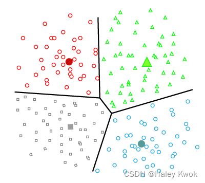
Partitioning Clustering

It is a type of clustering that divides the data into non-hierarchical groups. It is also known as the centroid-based method. The most common example of partitioning clustering is the K-Means Clustering algorithm.

Density-Based Clustering

The density-based clustering method connects the highly-dense areas into clusters, and the arbitrarily shaped distributions are formed as long as the dense region can be connected. This algorithm does it by identifying different clusters in the dataset and connects the areas of high densities into clusters. The dense areas in data space are divided from each other by sparser areas.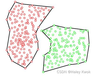

Distribution Model-Based Clustering

In the distribution model-based clustering method, the data is divided based on the probability of how a dataset belongs to a particular distribution. The grouping is done by assuming some distributions commonly Gaussian Distribution.

The example of this type is the Expectation-Maximization Clustering algorithm that uses Gaussian Mixture Models (GMM).

Hierarchical Clustering/ Agglomerative Hierarchical Clustering

In this technique, the dataset is divided into clusters to create a tree-like structure, which is also called a dendrogram. Hierarchical clustering is another unsupervised machine learning algorithm, which is used to group the unlabeled datasets into a cluster and also known as hierarchical cluster analysis or HCA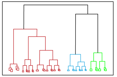

Fuzzy Clustering

Fuzzy clustering is a type of soft method in which a data object may belong to more than one group or cluster. Each dataset has a set of membership coefficients, which depend on the degree of membership to be in a cluster. Fuzzy C-means algorithm is the example of this type of clustering; it is sometimes also known as the Fuzzy k-means algorithm.

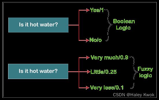
Photo Source

Association

Apriori Algorithm

This algorithm uses frequent datasets to generate association rules. It is designed to work on the databases that contain transactions. This algorithm uses a breadth-first search and Hash Tree to calculate the itemset efficiently.

It is mainly used for market basket analysis and helps to understand the products that can be bought together. It can also be used in the healthcare field to find drug reactions for patients.

Eclat Algorithm

Eclat algorithm stands for Equivalence Class Transformation. This algorithm uses a depth-first search technique to find frequent itemsets in a transaction database. It performs faster execution than Apriori Algorithm.

F-P Growth Algorithm

The F-P growth algorithm stands for Frequent Pattern, and it is the improved version of the Apriori Algorithm. It represents the database in the form of a tree structure that is known as a frequent pattern or tree. The purpose of this frequent tree is to extract the most frequent patterns.

---

Hyper Parameter Tuning

Approach 1: Use train_test_split and manually tune parameters by trial and error

from sklearn import svm, datasets
iris = datasets.load_iris()

import pandas as pd
df = pd.DataFrame(iris.data,columns=iris.feature_names)
df['flower'] = iris.target
df['flower'] = df['flower'].apply(lambda x: iris.target_names[x])
df[47:150]

from sklearn.model_selection import train_test_split
X_train, X_test, y_train, y_test = train_test_split(iris.data, iris.target, test_size=0.3)

model = svm.SVC(kernel='rbf',C=30,gamma='auto')
model.fit(X_train,y_train)
model.score(X_test, y_test)

# return
1

Approach 2: Use K Fold Cross validation

Manually try suppling models with different parameters to cross_val_score function with 5 fold cross validation

from sklearn.model_selection import cross_val_score

cross_val_score(svm.SVC(kernel='linear',C=10,gamma='auto'),iris.data, iris.target, cv=5)

cross_val_score(svm.SVC(kernel='rbf',C=10,gamma='auto'),iris.data, iris.target, cv=5)

cross_val_score(svm.SVC(kernel='linear',C=20,gamma='auto'),iris.data, iris.target, cv=5)
.....

Above approach is tiresome and very manual. We can use for loop as an alternative

import numpy as np

kernels = ['rbf', 'linear']
C = [1,10,20]
avg_scores = {}
for kval in kernels:
    for cval in C:
        cv_scores = cross_val_score(svm.SVC(kernel=kval,C=cval,gamma='auto'),iris.data, iris.target, cv=5)
        avg_scores[kval + '_' + str(cval)] = np.average(cv_scores)

avg_scores

# return
{'rbf_1': 0.9800000000000001,
 'rbf_10': 0.9800000000000001,
 'rbf_20': 0.9666666666666668,
 'linear_1': 0.9800000000000001,
 'linear_10': 0.9733333333333334,
 'linear_20': 0.9666666666666666}

From above results we can say that rbf with C=1 or 10 or linear with C=1 will give best performance

Approach 3: Use GridSearchCV

GridSearchCV does exactly same thing as for loop above but in a single line of code

from sklearn.model_selection import GridSearchCV
clf = GridSearchCV(svm.SVC(gamma='auto'), {
    'C': [1,10,20],                # parameter 
    'kernel': ['rbf','linear']
}, cv=5, return_train_score=False) 

clf.fit(iris.data, iris.target)
clf.cv_results_

df = pd.DataFrame(clf.cv_results_)
df

df[['param_C','param_kernel','mean_test_score']]

clf.best_params_

clf.best_score_

Another Example:

Use RandomizedSearchCV to reduce number of iterations and with random combination of parameters.

This is useful when you have too many parameters to try and your training time is longer. It helps reduce the cost of computation

from sklearn.model_selection import RandomizedSearchCV
rs = RandomizedSearchCV(svm.SVC(gamma='auto'), {
        'C': [1,10,20],
        'kernel': ['rbf','linear']
    }, 
    cv=5, 
    return_train_score=False, 
    n_iter=2
)
rs.fit(iris.data, iris.target)
pd.DataFrame(rs.cv_results_)[['param_C','param_kernel','mean_test_score']]

# return
	param_C	param_kernel	mean_test_score
0	1	linear	0.98
1	1	rbf	0.98

Different Models with Different Parameters

from sklearn import svm
from sklearn.ensemble import RandomForestClassifier
from sklearn.linear_model import LogisticRegression

model_params = {
    'svm': {
        'model': svm.SVC(gamma='auto'),
        'params' : {
            'C': [1,10,20],
            'kernel': ['rbf','linear']
        }  
    },
    'random_forest': {
        'model': RandomForestClassifier(),
        'params' : {
            'n_estimators': [1,5,10]
        }
    },
    'logistic_regression' : {
        'model': LogisticRegression(solver='liblinear',multi_class='auto'),
        'params': {
            'C': [1,5,10]
        }
    }
}

scores = []

for model_name, mp in model_params.items():
    clf =  GridSearchCV(mp['model'], mp['params'], cv=5, return_train_score=False)
    clf.fit(iris.data, iris.target)
    scores.append({
        'model': model_name,
        'best_score': clf.best_score_,
        'best_params': clf.best_params_
    })
    
df = pd.DataFrame(scores,columns=['model','best_score','best_params'])
df

# return
	model	best_score	best_params
0	svm	0.980000	{'C': 1, 'kernel': 'rbf'}
1	random_forest	0.960000	{'n_estimators': 5}
2	logistic_regression	0.966667	{'C': 5}

Another Example:

from sklearn import datasets
digits = datasets.load_digits()


from sklearn import svm
from sklearn.ensemble import RandomForestClassifier
from sklearn.linear_model import LogisticRegression
from sklearn.naive_bayes import GaussianNB
from sklearn.naive_bayes import MultinomialNB
from sklearn.tree import DecisionTreeClassifier

model_params = {
    'svm': {
        'model': svm.SVC(gamma='auto'),
        'params' : {
            'C': [1,10,20],
            'kernel': ['rbf','linear']
        }  
    },
    'random_forest': {
        'model': RandomForestClassifier(),
        'params' : {
            'n_estimators': [1,5,10]
        }
    },
    'logistic_regression' : {
        'model': LogisticRegression(solver='liblinear',multi_class='auto'),
        'params': {
            'C': [1,5,10]
        }
    },
    'naive_bayes_gaussian': {
        'model': GaussianNB(),
        'params': {}
    },
    'naive_bayes_multinomial': {
        'model': MultinomialNB(),
        'params': {}
    },
    'decision_tree': {
        'model': DecisionTreeClassifier(),
        'params': {
            'criterion': ['gini','entropy'],
            
        }
    }     
}

from sklearn.model_selection import GridSearchCV
import pandas as pd
scores = []

for model_name, mp in model_params.items():
    clf =  GridSearchCV(mp['model'], mp['params'], cv=5, return_train_score=False)
    clf.fit(digits.data, digits.target)
    scores.append({
        'model': model_name,
        'best_score': clf.best_score_,
        'best_params': clf.best_params_
    })
    
df = pd.DataFrame(scores,columns=['model','best_score','best_params'])
df


# return
	model	best_score	best_params
0	svm	0.949360	{'C': 1, 'kernel': 'linear'}
1	random_forest	0.899833	{'n_estimators': 10}
2	logistic_regression	0.920979	{'C': 1}
3	naive_bayes_gaussian	0.806344	{}
4	naive_bayes_multinomial	0.871452	{}
5	decision_tree	0.817474	{'criterion': 'entropy'}

K-Fold Cross Vaildation

# option 1 
# use all available data for training and testing on same dataset
# e.g., 100 math questions prepared, and a few questions to be tested
# option 2
# 70/100 for training and 30/100 for testing 

# option 3
# K-fold cross vaildation
# 1000 samples 20/100 for testing and 80/100 for training x 5 sets
# take average


from sklearn.linear_model import LogisticRegression
from sklearn.svm import SVC
from sklearn.ensemble import RandomForestClassifier
import numpy as np
from sklearn.datasets import load_digits
import matplotlib.pyplot as plt
digits = load_digits()

from sklearn.model_selection import train_test_split
X_train, X_test, y_train, y_test = train_test_split(digits.data,digits.target,test_size=0.3)

# Logistic Regression
lr = LogisticRegression(solver='liblinear',multi_class='ovr')
lr.fit(X_train, y_train)
lr.score(X_test, y_test)

# SVM
svm = SVC(gamma='auto')
svm.fit(X_train, y_train)
svm.score(X_test, y_test)

from sklearn.model_selection import cross_val_score

# cross_val_score uses stratifield kfold by default

# Logistic regression model performance using cross_val_score
cross_val_score(LogisticRegression(solver='liblinear',multi_class='ovr'), digits.data, digits.target,cv=3)

# svm model performance using cross_val_score
cross_val_score(SVC(gamma='auto'), digits.data, digits.target,cv=3)

# random forest performance using cross_val_score
cross_val_score(RandomForestClassifier(n_estimators=40),digits.data, digits.target,cv=3)

# Here we used cross_val_score to fine tune our random forest classifier and 
# figured that having around 40 trees in random forest gives best result.

n_estimators=[5,20,30,40]
average_scores ={}
for ne in n_estimators:
    cv_scores = cross_val_score(RandomForestClassifier(n_estimators=ne),digits.data, digits.target, cv=10)
    average_scores['the average score of' +'_'+str(ne)+'_'+'is'] = np.average(cv_scores)
average_scores

Bagging/ Ensemble Learning

Ensemble learning is all about using multiple models to combine their prediction power to get better predictions that has low variance. Bagging and boosting are two popular techniques that allows us to tackle high variance issue. In this video we will learn about bagging with simple visual demonstration. We will also right python code in sklearn to use BaggingClassifier.

from sklearn.preprocessing import StandardScaler

scaler = StandardScaler()
X_scaled = scaler.fit_transform(X)
X_scaled[:3]

from sklearn.model_selection import train_test_split

X_train, X_test, y_train, y_test = train_test_split(X_scaled, y, stratify=y, random_state=10)


from sklearn.model_selection import cross_val_score
from sklearn.tree import DecisionTreeClassifier

scores = cross_val_score(DecisionTreeClassifier(), X, y, cv=5)
scores

# return
0.7136575842458195

from sklearn.ensemble import BaggingClassifier

bag_model = BaggingClassifier(
    base_estimator=DecisionTreeClassifier(), 
    n_estimators=100, 
    max_samples=0.8, 
    oob_score=True,
    random_state=0
)
bag_model.fit(X_train, y_train)
bag_model.oob_score_

bag_model.score(X_test, y_test)


bag_model = BaggingClassifier(
    base_estimator=DecisionTreeClassifier(), 
    n_estimators=100, # use 100 datasets, trial and error
    max_samples=0.8, # 80% of my sample dataset
    oob_score=True, # out of bag, since the data is random, then you use sth data that does not appear to test
    random_state=0 # Controls the random resampling of the original dataset (sample wise and feature wise).
)
scores = cross_val_score(bag_model, X, y, cv=5)
scores

scores.mean()
# return
0.7578728461081402

# We can see some improvement in test score with bagging classifier as compared to a standalone classifier

from sklearn.ensemble import RandomForestClassifier

scores = cross_val_score(RandomForestClassifier(n_estimators=50), X, y, cv=5)
scores.mean()


# return
0.7669637551990494

from sklearn.svm import SVC
from sklearn.model_selection import cross_val_score

scores = cross_val_score(SVC(), X, y, cv=5)
scores.mean()

from sklearn.ensemble import BaggingClassifier

bag_model = BaggingClassifier(base_estimator=SVC(), n_estimators=100, max_samples=0.8, random_state=0)
scores = cross_val_score(bag_model, X, y, cv=5)
scores.mean()

---

References

Javapoint: Machine Learning

Scikit-learn