信号处理深度学习机器学习
机器学习性能与两种关键信号处理算法(快速傅里叶变换和最小均方预测)的有趣对比。 (A fun comparison of machine learning performance with two key signal processing algorithms — the Fast Fourier Transform and the Least Mean Squares prediction.)
Signal processing has given us a bag of tools that have been refined and put to very good use in the last fifty years. There is autocorrelation, convolution, Fourier and wavelet transforms, adaptive filtering via Least Mean Squares (LMS) or Recursive Least Squares (RLS), linear estimators, compressed sensing and gradient descent, to mention a few. Different tools are used to solve different problems, and sometimes, we use a combination of these tools to build a system to process signals.
信号处理为我们提供了一整套工具,这些工具在过去的五十年中已经完善并得到了很好的使用。 有自相关,卷积,傅立叶和小波变换,通过最小均方(LMS)或递归最小二乘(RLS)进行自适应滤波,线性估计器,压缩感测和梯度下降等。 使用不同的工具来解决不同的问题,有时,我们结合使用这些工具来构建用于处理信号的系统。
Machine Learning, or the deep neural networks, is much simpler to get used to because the underlying mathematics is fairly straightforward regardless of what network architecture we use. The complexity and the mystery of neural networks lie in the amount of data they process to get the fascinating results we currently have.
机器学习(即深度神经网络)要习惯得多,因为无论我们使用哪种网络架构,基础数学都非常简单明了。 神经网络的复杂性和奥秘在于它们处理的数据量,以获得我们目前拥有的迷人结果。
时间序列预测 (Time Series Prediction)
This article is an effort to compare the performance of a neural network for a few key signal processing algorithms. Let us look at time series prediction as the first example. We will implement a three layer sequential deep neural network to predict the next sample of a signal. We will also do it the traditional way by using a tap delay filter and adapting the weights based on the mean square error — this is the LMS filtering, an iterative approach to the optimal Weiner filter for estimating signal from noisy measurement. We will then compare the prediction error between the two methods. So, let us get started with writing the code!
本文旨在比较几种关键信号处理算法的神经网络性能。 让我们将时间序列预测作为第一个示例。 我们将实现一个三层顺序的深度神经网络,以预测信号的下一个样本。 我们还将通过使用抽头延迟滤波器并根据均方误差调整权重来实现传统方法-这是LMS滤波 ,这是一种针对最优Weiner滤波器的迭代方法,用于从噪声测量中估计信号。 然后,我们将比较两种方法之间的预测误差。 因此,让我们开始编写代码!
Let us first import all the usual python libraries we need. Since we are going to be using the TensorFlow and Keras framework, we will import them too.
让我们首先导入我们需要的所有常用python库。 由于我们将使用TensorFlow和Keras框架,因此我们也将其导入。
神经网络预测 (Prediction with Neural Networks)
Let us start building our 3 layer Neural network now. The input layer takes 64 samples and produces 32 samples. The hidden layer maps these 32 outputs from the first layer to 8 samples. The final layer maps these 8 samples in to 1 predicted output. Remember that the input size is provided with the input_shape parameter in the first layer.
现在让我们开始构建3层神经网络。 输入层获取64个样本,并产生32个样本。 隐藏层将这32个输出从第一层映射到8个样本。 最后一层将这8个样本映射为1个预测输出。 请记住,输入大小随第一层的input_shape参数提供。
We will use the Adam optimizer without bothering about what it is. That is the benefit of TensorFlow, we don’t need to know every detail about all the processing required for neural network to build one using this amazing framework. If we find out that the Adam optimizer doesn’t work as well, we will simply try another optimizer — RMSprop for example.
我们将使用Adam优化器而不用担心它是什么。 这就是TensorFlow的好处,我们不需要了解神经网络使用此惊人框架构建一个神经网络所需的所有处理的每个细节。 如果发现Adam优化器不能正常工作,我们将简单地尝试另一个优化器 -例如RMSprop。
Let us now create a time series, a simple superposition of sine waves. We will then add noise to it to mimic a real world signal.
现在让我们创建一个时间序列,一个正弦波的简单叠加。 然后,我们将向其添加噪声以模拟现实世界的信号。
Now that we have the data, let us think about how to feed this data to the neural network for training. We know the network takes 64 samples at the input and produces one output sample. Since we want to train the network to predict the next sample, we want to use the 65th sample as the output label.
现在我们有了数据,让我们考虑如何将这些数据馈送到神经网络进行训练。 我们知道网络在输入处获取64个样本,并生成一个输出样本。 由于我们要训练网络以预测下一个样本,因此我们希望将第65个样本用作输出标签。
The first input set is therefore from sample 0 to sample 63 (the first 64 samples) and the first label is sample 64 (the 65th sample). The second input set can either be a separate set of 64 samples (non-overlapping window), or we can choose to have a sliding window and take 64 samples from sample 1 to sample 64. Let us follow the sliding window approach, just to generate a lot of training data from the time series we have.
因此,第一个输入集是从样本0到样本63(前64个样本),而第一个标签是样本64(第65个样本)。 第二个输入集可以是64个样本的单独集合(不重叠的窗口),也可以选择有一个滑动窗口并从样本1到64取64个样本。让我们遵循滑动窗口的方法,从我们拥有的时间序列中生成很多训练数据。
Also note that we are using the noisy samples as the input while using the noiseless data as the label. We want the neural network to predict the actual signal even in presence of noise.
还要注意,我们将噪声样本用作输入,而将无噪声数据用作标签。 我们希望神经网络即使在存在噪声的情况下也能预测实际信号。
Let us look at the sizes of the time series data and the training data. See that we generated 5000 samples for our time series data, but we created 3935 x 64 = 251840 samples of input data to our neural network.
让我们看一下时间序列数据和训练数据的大小。 看到我们为时间序列数据生成了5000个样本,但是我们为神经网络创建了3935 x 64 = 251840个输入数据样本。
The shape of train_data is the number of input sets x input length. Here, we have 3935 batches of input, each input being 64 samples long.
train_data的形状是输入集的数量x输入长度。 在这里,我们有3935批输入,每个输入长64个样本。
print(y.shape, train_data.shape, train_labels.shape)(5000,) (3935, 64) (3935,)We are now ready to train the neural network. Let us instantiate the model first. The model summary provides information on how many layers, what is the output shape, and the number of parameters we need to train for this neural network.
现在我们准备训练神经网络。 让我们首先实例化模型。 该模型摘要提供了有关此神经网络需要训练的层数,输出形状以及参数数量的信息。
For the first layer, we have 64 inputs and 32 outputs. A dense layer implemets the equation y = f(Wx + b), where f is the activation function, W is the weight matrix and b is the bias. We can immediately see that W is a 64 x 32 matrix, and b is a 32 x 1 vector. This gives us 32 x 64 + 32 = 2080 parameters to train for the first layer. The reader can do similar computations to verify the parameters for second and third layer, as an exercise in understanding. After all, you wouldn’t be reading this article unless you are a beginner to Machine Learning and eager to get started :)
对于第一层,我们有64个输入和32个输出。 致密层实现等式y = f(Wx + b) ,其中f是激活函数, W是权重矩阵, b是偏差。 我们可以立即看到W是64 x 32的矩阵, b是32 x 1的向量。 这给我们提供了32 x 64 + 32 = 2080个参数来训练第一层。 读者可以进行类似的计算以验证第二层和第三层的参数,作为理解的练习。 毕竟,除非您是机器学习的初学者并且渴望入门,否则您将不会阅读本文:)
model = dnn_keras_tspred_model()Model: "sequential"
_________________________________________________________________
Layer (type)                 Output Shape              Param #
=================================================================
dense (Dense)                (None, 32)                2080
_________________________________________________________________
dense_1 (Dense)              (None, 8)                 264
_________________________________________________________________
dense_2 (Dense)              (None, 1)                 9
=================================================================
Total params: 2,353
Trainable params: 2,353
Non-trainable params: 0
_________________________________________________________________
Alright, onward to training then. Since we are using the Keras framework, training is as simple as calling the fit() method. With TensorFlow, we need to do a little more work, but that is for another article.
好吧,那就继续训练吧。 由于我们使用的是Keras框架,因此培训就像调用fit()方法一样简单。 使用TensorFlow,我们需要做更多的工作,但这是另一篇文章。
Let us use 100 epochs, which just means that we will use the same training data again and again to train the neural network and will do so 100 times. In each epoch, the network uses the number of batches of input and label sets to train the parameters.
让我们使用100个纪元 ,这意味着我们将一次又一次地使用相同的训练数据来训练神经网络,并且将进行100次。 在每个纪元中,网络使用输入和标签集的批次数量来训练参数。
Let us use the datetime to profile how long this training takes, and the history value that is returned as a Python Dictionary to get the validation loss after each epoch.
让我们使用日期时间来描述该训练需要多长时间,并使用历史记录值作为Python字典返回,以获取每个时期后的验证损失。
DNN training done. Time elapsed: 10.177171 s
Now that the network is trained, and we see that the validation loss has decreased over epochs to the point that it has flattened out (indicating further training doesn’t yield any significant improvements), let us use this network to see how well it performs against test data.
既然已经对网络进行了培训,并且我们看到验证损失已经减少了几步,直到达到平坦为止(表明进一步的培训不会带来任何明显的改善),让我们使用该网络来查看其效果如何根据测试数据。
Let us create the test data set exactly the same way as we created the training data sets, but use only that part of the time series that we have not used for training before. We want to surprise the neural network with data it has not seen before to know how well it can perform.
让我们创建测试数据集的方式与创建训练数据集的方式完全相同,但是只使用时间序列中我们从未用于训练的那部分。 我们想用之前从未见过的数据让神经网络感到惊讶,以了解其性能如何。
We will now call the predict() method in Keras framework to get the outputs of the neural network for the test data set. This step is different if we use the TensorFlow framework, but we will cover that in another article.
现在,我们将在Keras框架中调用predict()方法,以获取测试数据集的神经网络输出。 如果我们使用TensorFlow框架,则此步骤有所不同,但我们将在另一篇文章中介绍。
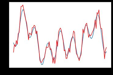
As we see, the prediction from neural network is very close to the actual noise free data!
如我们所见,来自神经网络的预测非常接近实际的无噪声数据!

LMS算法的预测 (Prediction with LMS algorithm)
We will use a L=64 tap filter to predict the next sample. We don’t need that large a filter, but let us keep the number of inputs per output sample same as what we used for neural network.
我们将使用L = 64抽头滤波器来预测下一个样本。 我们不需要那么大的滤波器,但让我们将每个输出样本的输入数量保持与用于神经网络的数量相同。
The filter coefficients (or weights) are obtained by computing the error between predicted and measured sample, and adjusting the weights based on the correlation between mean square error and the input measurements.
滤波器系数(或权重)是通过计算预测样本和测量样本之间的误差,并基于均方误差和输入测量值之间的相关性来调整权重而获得的。
As you see in the code, yrlms[k] is the filter output when the inputs are ypn[k-L:k], the error is computed as the difference between the noisy measured value ypn[k] and the filter output yrlms[k]. The correlation between measurement and error is given by the product of ypn[k-L:k] and e, and mu is the LMS step size (or learning rate).
如您在代码中看到的, yrlms [k]是输入为ypn [kL:k]时的滤波器输出,误差计算为噪声测量值ypn [k]与滤波器输出yrlms [k]之差 。 测量和误差之间的相关性由ypn [kL:k]与e的乘积给出,而mu是LMS步长(或学习率)。
As we see, the LMS prediction is equally good, despite having much lower complexity.
如我们所见,尽管LMS预测的复杂度要低得多,但它同样好。
(64,) (1064,)
LMS和神经网络之间的预测结果比较 (Comparing Prediction Results between LMS and Neural Network)
Before we close this section, let us compare the error between LMS prediction and the neural network prediction. To be fair, I ignored the initial portion of the LMS to give it time to converge when measuring the mean square error and SNR. Despute that, we see that the neural network performance is 5 dB better than the LMS performance!
在结束本节之前,让我们比较LMS预测和神经网络预测之间的误差。 公平地说,我忽略了LMS的初始部分,以便在测量均方误差和SNR时有时间收敛。 对此,我们看到神经网络性能比LMS性能好5 dB!

Neural network SNR: 19.986311477279084
LMS Prediction SNR: 14.93359076022336
快速傅立叶变换 (Fast Fourier Transform)
Alright, a neural network beat LMS by 5 dB in signal prediction, but let us see if a neural network can be trained to do the Fourier Transform. We will compare it to the FFT (Fast Fourier Transform) from SciPy FFTPack. The FFT algorithm is at the heart of signal processing, can the neural network be trained to mimic that too? Let us find out…
好了,神经网络在信号预测方面比LMS胜5 dB,但让我们看看是否可以训练神经网络进行傅立叶变换。 我们将其与SciPy FFTPack的FFT(快速傅立叶变换)进行比较。 FFT算法是信号处理的核心,是否可以训练神经网络来模仿它? 让我们找出……
We will use the same signal we created before, the superposition of sine waves, to evaluate FFT as well. Let us look at the FFT ouput first.
我们将使用之前创建的相同信号(正弦波的叠加)来评估FFT。 首先让我们看一下FFT输出。

Let us create a neural network model to mimic the FFT now. In contrast to the model we created before where we have 64 inputs but only one output, this model needs to generate 64 outputs for every 64 sample input set.
让我们创建一个神经网络模型来模拟FFT。 与之前创建的具有64个输入但只有一个输出的模型相比,该模型需要为每64个样本输入集生成64个输出。
And since FFT inputs and outputs are complex, we need twice the number of samples at the input, arranged as real followed by imaginary. Since the outputs are also complex, we again 2 x NFFT samples.
而且由于FFT的输入和输出很复杂,因此我们需要在输入处添加两倍数量的采样,按实数排列,然后按虚数排列。 由于输出也很复杂,因此我们再次进行2 x NFFT采样。
To train this neural network model, let us use random data generated using numpy.random.normal and set the labels based on the FFT routine from the SciPy FFTPack that we are comparing with.
为了训练该神经网络模型,让我们使用使用numpy.random.normal生成的随机数据,并根据与之比较的SciPy FFTPack中的FFT例程设置标签。
The rest of the code is fairly similar to the previous neural network training. Here, I am running 10,000 batches at a time, and I have an outer for loop to do multiple sets of 10,000 batches if the network needs more training. Note that this needs the model to be created outside the for loop, so that the weights are not reinitialized.
其余代码与先前的神经网络训练非常相似。 在这里,我一次运行10,000个批次,并且如果网络需要更多培训,我有一个外部for循环可以执行多组10,000个批次。 请注意,这需要在for循环之外创建模型,以便不会重新初始化权重。
See from model summary that there are almost 50,000 parameters for just a 64 point FFT. We can reduce this a bit since we are only evaluating real inputs while keeping the imaginary parts as zero, but the goal here is to quickly compare if the neural network can be trained to do the Fourier Transform.
从模型摘要中可以看出,仅64点FFT就有近50,000个参数。 我们可以减少一点,因为我们只评估实数输入,而将虚部保持为零,但是这里的目标是快速比较神经网络是否可以训练以进行傅立叶变换。
Model: "sequential_1"
_________________________________________________________________
Layer (type)                 Output Shape              Param #
=================================================================
dense_3 (Dense)              (None, 128)               16512
_________________________________________________________________
dense_4 (Dense)              (None, 128)               16512
_________________________________________________________________
dense_5 (Dense)              (None, 128)               16512
=================================================================
Total params: 49,536
Trainable params: 49,536
Non-trainable params: 0
_________________________________________________________________
DNN training done. Time elapsed:  30.64511 s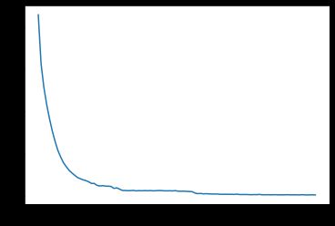
Training is done. Let us now test the network using the same input samples we created for LMS. We compare the neural network output to the FFT ouput and they are identical! How amazing is that!
培训完成。 现在让我们使用为LMS创建的相同输入样本来测试网络。 我们将神经网络输出与FFT输出进行比较,它们是相同的! 那太神奇了!

Let us do one last evaluation before we conclude this article. We will compare the neural network output with the FFT output for some random input data, and see how the mean square error and SNR looks like.
在结束本文之前,让我们做最后一个评估。 对于某些随机输入数据,我们将神经网络输出与FFT输出进行比较,并查看均方误差和SNR的样子。
Running the code below, we get a decent 23.64 dB SNR. While we do see some samples every now and then where the error is high, for most part, the error is very small. Given that we trained the neural network for only 10,000 batches, this is a pretty good result!
运行下面的代码,我们得到不错的23.64 dB SNR。 虽然我们时不时会看到一些样本,但误差很大,但在大多数情况下,误差很小。 鉴于我们只训练了10,000个批次的神经网络,这是一个相当不错的结果!

Neural Network SNR compared to SciPy FFT: 23.64254974707859摘要 (Summary)
Being stuck inside during Covid-19, it was a fun weekend project to compare machine learning performance to some key signal processing algorithms. We see that machine learning can do what signal processing can, but has inherently higher complexity, with the benefit of being generalizable to different problems. The signal processing algorithms are optimal for the job in terms of complexity, but are specific to the particular problems they solve. We can’t use FFT in place of LMS or vice versa, while we can use the same neural network processor, and just load a different set of weights to solve a different problem. That is the versatility of neural networks.
被困在Covid-19大会期间,这是一个有趣的周末项目,旨在将机器学习性能与一些关键信号处理算法进行比较。 我们看到机器学习可以完成信号处理所能完成的工作,但是固有地具有更高的复杂度,其优点是可以推广到不同的问题。 信号处理算法在复杂性方面最适合该工作,但是特定于它们解决的特定问题。 我们不能使用FFT代替LMS,反之亦然,而我们可以使用相同的神经网络处理器,而只是加载不同的权重集来解决不同的问题。 那就是神经网络的多功能性。
And with that note, I’ll conclude this article. I hope you had as much fun reading this as I had putting this together. Please leave your feedback too if you found it helpful and learnt a thing or two!
有了这个注释,我将结束本文。 希望您阅读这些内容和我整理这些内容一样开心。 如果您觉得有帮助并且学到了一两件事,也请留下您的反馈!
翻译自: https://towardsdatascience.com/machine-learning-and-signal-processing-103281d27c4b
信号处理深度学习机器学习