Machine Learning 04 - Neural Networks

正在学习Stanford吴恩达的机器学习课程，常做笔记，以便复习巩固。
鄙人才疏学浅，如有错漏与想法，还请多包涵，指点迷津。

Week 04

4.1 Model Representation

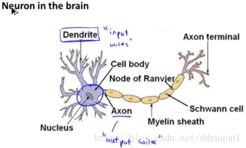
4.1.1 Origin of model

Neural network be modelled from the neuron in the brain.

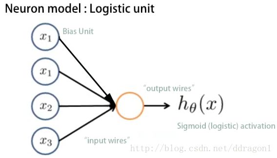
4.1.2 Logistic unit

A basic model of neural network is as follow :

Remark :

x=⎡⎣⎢⎢⎢x0x1x2x3⎤⎦⎥⎥⎥,θ=⎡⎣⎢⎢⎢θ0θ1θ2θ3⎤⎦⎥⎥⎥ x = [ x 0 x 1 x 2 x 3 ] , θ = [ θ 0 θ 1 θ 2 θ 3 ]

θ θ is also called “weights” in neural networks.

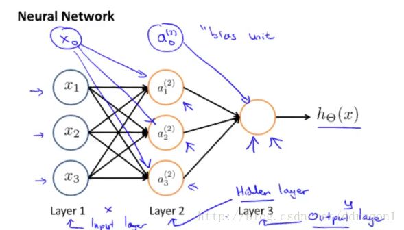
4.1.3 Neural network

(1) Schematic diagram

Symbol

sj s j - the number of the units in layer j j ， not counting bias unit.

a(j)i a i ( j ) - “activation” of unit i i in layer j j

Θ(j) Θ ( j ) - matrix of weights controlling function mapping from layer j j to layer j+1 j + 1 , with dimension of sj+1×(sj+1) s j + 1 × ( s j + 1 )

L L - total number of layers in network

(2) Mathematical representation

Layer 2

a(2)1=g(Θ(1)10x0+Θ(1)11x1+Θ(1)12x2+Θ(1)13x3)a(2)2=g(Θ(1)20x0+Θ(1)21x1+Θ(1)22x2+Θ(1)23x3)a(2)3=g(Θ(1)30x0+Θ(1)31x1+Θ(1)32x2+Θ(1)33x3) a 1 ( 2 ) = g ( Θ 10 ( 1 ) x 0 + Θ 11 ( 1 ) x 1 + Θ 12 ( 1 ) x 2 + Θ 13 ( 1 ) x 3 ) a 2 ( 2 ) = g ( Θ 20 ( 1 ) x 0 + Θ 21 ( 1 ) x 1 + Θ 22 ( 1 ) x 2 + Θ 23 ( 1 ) x 3 ) a 3 ( 2 ) = g ( Θ 30 ( 1 ) x 0 + Θ 31 ( 1 ) x 1 + Θ 32 ( 1 ) x 2 + Θ 33 ( 1 ) x 3 )

Layer 3

hΘ(x)=a(3)1=g(Θ(2)10a(2)0+Θ(2)11a(2)1+Θ(2)12a(2)2+Θ(2)13a(2)3) h Θ ( x ) = a 1 ( 3 ) = g ( Θ 10 ( 2 ) a 0 ( 2 ) + Θ 11 ( 2 ) a 1 ( 2 ) + Θ 12 ( 2 ) a 2 ( 2 ) + Θ 13 ( 2 ) a 3 ( 2 ) )

(3) Vectorization

Layer 1

a(1)=⎡⎣⎢⎢⎢⎢⎢⎢a(1)0a(1)1a(1)2a(1)3⎤⎦⎥⎥⎥⎥⎥⎥=⎡⎣⎢⎢⎢x0x1x2x3⎤⎦⎥⎥⎥=x a ( 1 ) = [ a 0 ( 1 ) a 1 ( 1 ) a 2 ( 1 ) a 3 ( 1 ) ] = [ x 0 x 1 x 2 x 3 ] = x

Layer 2

a(2)=⎡⎣⎢⎢⎢a(2)1a(2)2a(2)3⎤⎦⎥⎥⎥=⎡⎣⎢⎢⎢g(z(2)1)g(z(2)2)g(z(2)3)⎤⎦⎥⎥⎥=g(⎡⎣⎢⎢⎢z(2)1z(2)2z(2)3⎤⎦⎥⎥⎥)=g(z(2))=g(Θ(1)a(1))=g(⎡⎣⎢⎢⎢Θ(1)10x0+Θ(1)11x1+Θ(1)12x2+Θ(1)13x3Θ(1)20x0+Θ(1)21x1+Θ(1)22x2+Θ(1)23x3Θ(1)30x0+Θ(1)31x1+Θ(1)32x2+Θ(1)33x3⎤⎦⎥⎥⎥)=⎡⎣⎢⎢⎢g(Θ(1)10x0+Θ(1)11x1+Θ(1)12x2+Θ(1)13x3)g(Θ(1)20x0+Θ(1)21x1+Θ(1)22x2+Θ(1)23x3)g(Θ(1)30x0+Θ(1)31x1+Θ(1)32x2+Θ(1)33x3)⎤⎦⎥⎥⎥ a ( 2 ) = [ a 1 ( 2 ) a 2 ( 2 ) a 3 ( 2 ) ] = [ g ( z 1 ( 2 ) ) g ( z 2 ( 2 ) ) g ( z 3 ( 2 ) ) ] = g ( [ z 1 ( 2 ) z 2 ( 2 ) z 3 ( 2 ) ] ) = g ( z ( 2 ) ) = g ( Θ ( 1 ) a ( 1 ) ) = g ( [ Θ 10 ( 1 ) x 0 + Θ 11 ( 1 ) x 1 + Θ 12 ( 1 ) x 2 + Θ 13 ( 1 ) x 3 Θ 20 ( 1 ) x 0 + Θ 21 ( 1 ) x 1 + Θ 22 ( 1 ) x 2 + Θ 23 ( 1 ) x 3 Θ 30 ( 1 ) x 0 + Θ 31 ( 1 ) x 1 + Θ 32 ( 1 ) x 2 + Θ 33 ( 1 ) x 3 ] ) = [ g ( Θ 10 ( 1 ) x 0 + Θ 11 ( 1 ) x 1 + Θ 12 ( 1 ) x 2 + Θ 13 ( 1 ) x 3 ) g ( Θ 20 ( 1 ) x 0 + Θ 21 ( 1 ) x 1 + Θ 22 ( 1 ) x 2 + Θ 23 ( 1 ) x 3 ) g ( Θ 30 ( 1 ) x 0 + Θ 31 ( 1 ) x 1 + Θ 32 ( 1 ) x 2 + Θ 33 ( 1 ) x 3 ) ]

Layer 3

hΘ(x)=a(3)=g(z(3))=g(Θ(2)a(2))=g(Θ(2)10a(2)0+Θ(2)11a(2)1+Θ(2)12a(2)2+Θ(2)13a(2)3) h Θ ( x ) = a ( 3 ) = g ( z ( 3 ) ) = g ( Θ ( 2 ) a ( 2 ) ) = g ( Θ 10 ( 2 ) a 0 ( 2 ) + Θ 11 ( 2 ) a 1 ( 2 ) + Θ 12 ( 2 ) a 2 ( 2 ) + Θ 13 ( 2 ) a 3 ( 2 ) )

Remark :

hΘ(x)∈[0,1] h Θ ( x ) ∈ [ 0 , 1 ] is not a logstic function compare to the logistic regression.

The key of the vectorization is a(j)=g(z(j))=g(Θ(j−1)a(j−1)) a ( j ) = g ( z ( j ) ) = g ( Θ ( j − 1 ) a ( j − 1 ) ) , it likes a “loop”.

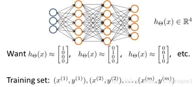
4.1.4 Multiclass classification

To classify data into multiple types, let the hypothesis function return a vector of values.

Simlarly, using one-vs-all method to solve the mutiple classfication problem.

The multiple output units :

4.2 Backpropagation

4.2.1 Cost function

Review the cost function of logistic regression :

J(θ)=−1m[∑i=1m(y(i)loghθ(x(i))+(1−y(i))log(1−hθ(x(i)))]+λ2m∑j=1nθ2j J ( θ ) = − 1 m [ ∑ i = 1 m ( y ( i ) l o g h θ ( x ( i ) ) + ( 1 − y ( i ) ) l o g ( 1 − h θ ( x ( i ) ) ) ] + λ 2 m ∑ j = 1 n θ j 2

In neural network, we have K K output, that is

hΘ(x)∈RK(hΘ(x))i=ithoutput h Θ ( x ) ∈ R K ( h Θ ( x ) ) i = i t h output

then the cost function of neural network is the sum of all K K logistic cost function :

J(Θ)=−1m∑i=1m∑k=1K[y(i)klog((hΘ(x(i)))k)+(1−y(i)k)log((1−hΘ(x(i)))k)]+λ2m∑l=1L−1∑i=1sl+1∑j=1sl(Θ(l)ij)2 J ( Θ ) = − 1 m ∑ i = 1 m ∑ k = 1 K [ y k ( i ) l o g ( ( h Θ ( x ( i ) ) ) k ) + ( 1 − y k ( i ) ) l o g ( ( 1 − h Θ ( x ( i ) ) ) k ) ] + λ 2 m ∑ l = 1 L − 1 ∑ i = 1 s l + 1 ∑ j = 1 s l ( Θ i j ( l ) ) 2

Remark : in the regulation part, the columns inludes the bias unit, the rows exclude the bias unit.

4.2.2 Gradient of cost function and algorithm

Io order to use gradient descent or other algorithm, we need to compute J(Θ) J ( Θ ) and ∂∂Θ(l)ijJ(Θ) ∂ ∂ Θ i j ( l ) J ( Θ )

Let

δL=a(L)−y;δ(i)=Θ(i)Tδ(j).∗g′(z(i)),2≤i≤L−1 δ L = a ( L ) − y ; δ ( i ) = Θ ( i ) T δ ( j ) . ∗ g ′ ( z ( i ) ) , 2 ≤ i ≤ L − 1

(for a detailed deducing, there is a reference material BP算法的推导过程)

then

∂∂Θ(l)ijJ(Θ)=a(l)jδ(l+1)i,(λ=0) ∂ ∂ Θ i j ( l ) J ( Θ ) = a j ( l ) δ i ( l + 1 ) , ( λ = 0 )

• Backpropagation algorithm for neural network - Algorthm 3

Training set {(x(1),y(1)),⋯,(x(m),y(m))} { ( x ( 1 ) , y ( 1 ) ) , ⋯ , ( x ( m ) , y ( m ) ) }
Set Δ(l)ij=0 for all l,i,j Δ i j ( l ) = 0  for all  l , i , j
For i=1 i = 1 to m m
Set a(1)=x(i) a ( 1 ) = x ( i )
Perform forward propagation to compute a(l) a ( l ) for l=2,3,⋯,L l = 2 , 3 , ⋯ , L
Using y(i) y ( i ) , compute δ(L)=a(L)−y(i) δ ( L ) = a ( L ) − y ( i )
Compute δ(L−1),δ(L−2),⋯,δ(2) δ ( L − 1 ) , δ ( L − 2 ) , ⋯ , δ ( 2 )
Δ(l):=Δ(l)+δ(l+1)(a(l))T Δ ( l ) := Δ ( l ) + δ ( l + 1 ) ( a ( l ) ) T
D(l)ij:=1m(Δ(l)ij+λΘ(l)ij), if j≠0 D i j ( l ) := 1 m ( Δ i j ( l ) + λ Θ i j ( l ) ) ,  if  j ≠ 0
D(l)ij:=1mΔ(l)ij                 ,  if j=0 D i j ( l ) := 1 m Δ i j ( l )                                   ,    if  j = 0
method of SGD

Thus we get ∂∂Θ(l)ijJ(Θ)=D(l)ij ∂ ∂ Θ i j ( l ) J ( Θ ) = D i j ( l ) .

4.3 Implement in Practice

4.3.1 Unrolling paramrters

With neural network, we are working with sets of matrices, in order to use advanced optimization function, we need to transform them into one long vector.

Code : unroll

thetaVector = [ Theta1(:); Theta2(:); Theta3(:); ]
deltaVector = [D1(:); D2(:); D3(:)]

Code : roll

Theta1 = reshape(thetaVector(1:110), 10, 11)
Theta2 = reshape(thetaVector(111:220), 10, 11)
Thera3 = reshape(thetaVector(221:231), 1, 11)

4.3.2 Gradient checking

In order to assure that our backpropagation works as intended, we need to check the gradient.

We can approximate the derivative of our cost function with:

∂J(Θ)∂Θ(j)≈J(Θ(j)1,⋯,Θ(j)k+ϵ,Θ(j)n)−J(Θ(j)1,⋯,Θ(j)k−ϵ,Θ(j)n)2ϵ ∂ J ( Θ ) ∂ Θ ( j ) ≈ J ( Θ 1 ( j ) , ⋯ , Θ k ( j ) + ϵ , Θ n ( j ) ) − J ( Θ 1 ( j ) , ⋯ , Θ k ( j ) − ϵ , Θ n ( j ) ) 2 ϵ

The ϵ ϵ is usually set 10−4 10 − 4 to guarantee the accuracy.

Code

epsilon = 1e-4;
for i:n
    thetaPlus = theta;
    thetaPlus += epsilon;
    thetaMinus = theta;
    thetaMinuw += epsilon;
    gradApprox(i) = (J(thetaPlus) - J(thetaMinus)) / (2*epsilon)
end

4.3.3 Random initialization

Initialize all theta weights to zero cause symmetry breaking, we can randomly initialize theta.

Initialize each Θ(l)ij Θ i j ( l ) to a random value between [−ϵ,ϵ] [ − ϵ , ϵ ] .

Code

Theta1 = ran(10,11)*(2*INIT_EPSILON)-INIT_EPSILON;
Theta2 = rand(1,11)*(2*INIT_EPSILON)-INIT_EPSILON;
...

4.4 Summary

Pick a Network Architecture

• number of input units = dimension of features x(i) x ( i )
• number of output units = number of classes
• number of hidden units per layer = ususlly more is better (must balance with cost function computation)

Training a Neural Network

• Randomly initialize the weights
• Implement forward propagation
• Implement the cost function
• Implement backpropagation
• Gradient checking (remember to disable checking)
• Use gradient descent or built-in optimization function