pray_HKY2002

鲍鱼数据案例（岭回归、LASSO回归）

鲍鱼数据集案例实战）

数据集探索性分析
鲍鱼数据预处理
对sex特征进行OneHot编码，便于后续模型纳入哑变量
筛选特征
将鲍鱼数据集划分为训练集和测试集
实现线性回归和岭回归
使用numpy实现线性回归
使用sklearn实现线性回归
使用Numpy实现岭回归
利用sklearn实现岭回归
岭迹分析
使用LASSO构建鲍鱼年龄预测模型
LASSO的正则化路径
残差图

数据集探索性分析

import pandas as pd
import warnings
warnings.filterwarnings('ignore')
data=pd.read_csv(r"E:\大二下\机器学习实践\abalone_dataset.csv")
data.head()

	sex	length	diameter	height	whole weight	shucked weight	viscera weight	shell weight	rings
0	M	0.455	0.365	0.095	0.5140	0.2245	0.1010	0.150	15
1	M	0.350	0.265	0.090	0.2255	0.0995	0.0485	0.070	7
2	F	0.530	0.420	0.135	0.6770	0.2565	0.1415	0.210	9
3	M	0.440	0.365	0.125	0.5160	0.2155	0.1140	0.155	10
4	I	0.330	0.255	0.080	0.2050	0.0895	0.0395	0.055	7

#查看数据集中样本数量和特征数量
data.shape

(4177, 9)

#查看数据信息，检查是否有缺失值
data.info()


RangeIndex: 4177 entries, 0 to 4176
Data columns (total 9 columns):
sex               4177 non-null object
length            4177 non-null float64
diameter          4177 non-null float64
height            4177 non-null float64
whole weight      4177 non-null float64
shucked weight    4177 non-null float64
viscera weight    4177 non-null float64
shell weight      4177 non-null float64
rings             4177 non-null int64
dtypes: float64(7), int64(1), object(1)
memory usage: 293.8+ KB

data.describe()

	length	diameter	height	whole weight	shucked weight	viscera weight	shell weight	rings
count	4177.000000	4177.000000	4177.000000	4177.000000	4177.000000	4177.000000	4177.000000	4177.000000
mean	0.523992	0.407881	0.139516	0.828742	0.359367	0.180594	0.238831	9.933684
std	0.120093	0.099240	0.041827	0.490389	0.221963	0.109614	0.139203	3.224169
min	0.075000	0.055000	0.000000	0.002000	0.001000	0.000500	0.001500	1.000000
25%	0.450000	0.350000	0.115000	0.441500	0.186000	0.093500	0.130000	8.000000
50%	0.545000	0.425000	0.140000	0.799500	0.336000	0.171000	0.234000	9.000000
75%	0.615000	0.480000	0.165000	1.153000	0.502000	0.253000	0.329000	11.000000
max	0.815000	0.650000	1.130000	2.825500	1.488000	0.760000	1.005000	29.000000

#观察sex列的取值的分布情况
import seaborn as sns
import matplotlib.pyplot as plt
%matplotlib inline

sns.countplot(x = "sex",data=data)

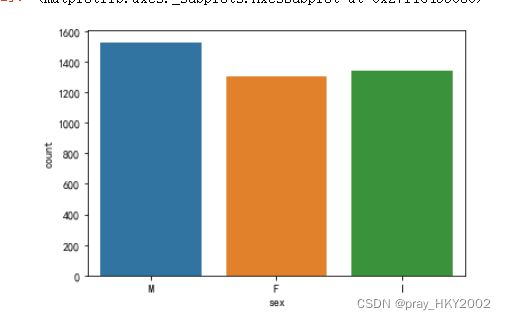
data['sex'].value_counts()

M    1528
I    1342
F    1307
Name: sex, dtype: int64

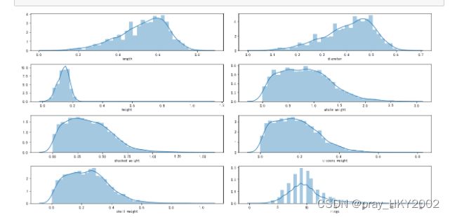
i=1 #子图计数
plt.figure(figsize=(16,8))
for col in data.columns[1:]:
    plt.subplot(4,2,i)
    i = i + 1
    sns.distplot(data[col])
plt.tight_layout()

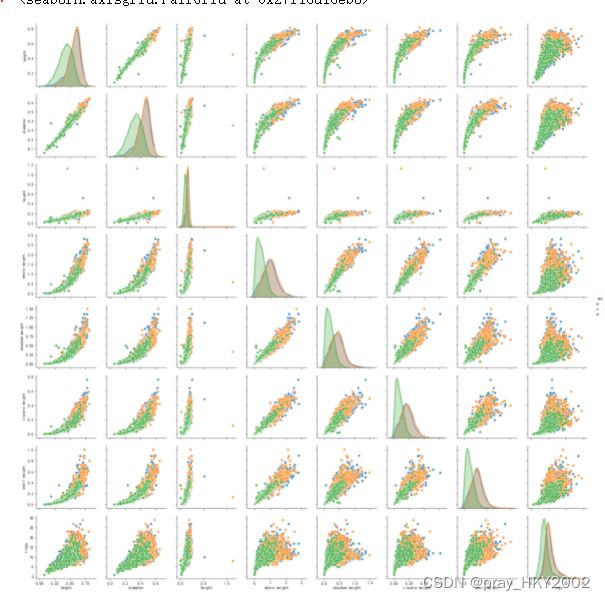
sns.pairplot(data,hue="sex")

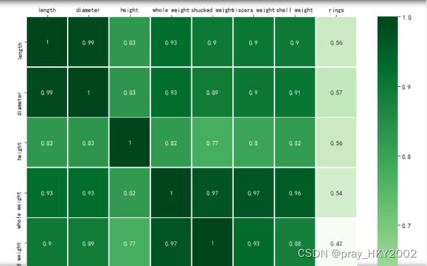
corr_df = data.corr()
corr_df

	length	diameter	height	whole weight	shucked weight	viscera weight	shell weight	rings
length	1.000000	0.986812	0.827554	0.925261	0.897914	0.903018	0.897706	0.556720
diameter	0.986812	1.000000	0.833684	0.925452	0.893162	0.899724	0.905330	0.574660
height	0.827554	0.833684	1.000000	0.819221	0.774972	0.798319	0.817338	0.557467
whole weight	0.925261	0.925452	0.819221	1.000000	0.969405	0.966375	0.955355	0.540390
shucked weight	0.897914	0.893162	0.774972	0.969405	1.000000	0.931961	0.882617	0.420884
viscera weight	0.903018	0.899724	0.798319	0.966375	0.931961	1.000000	0.907656	0.503819
shell weight	0.897706	0.905330	0.817338	0.955355	0.882617	0.907656	1.000000	0.627574
rings	0.556720	0.574660	0.557467	0.540390	0.420884	0.503819	0.627574	1.000000

fig ,ax =plt.subplots(figsize=(12,12))
##绘制热力图
ax = sns.heatmap(corr_df,linewidths=.5,
                cmap="Greens",
                annot=True,
                xticklabels=corr_df.columns,
                yticklabels=corr_df.index)
ax.xaxis.set_label_position('top')
ax.xaxis.tick_top()

鲍鱼数据预处理

对sex特征进行OneHot编码，便于后续模型纳入哑变量

#只用pandas的get_dummies函数对sex特征做OneHot编码处理
sex_onehot = pd.get_dummies(data["sex"],prefix="sex")
data[sex_onehot.columns] = sex_onehot
data.head()

	sex	length	diameter	height	whole weight	shucked weight	viscera weight	shell weight	rings	sex_F	sex_I	sex_M
0	M	0.455	0.365	0.095	0.5140	0.2245	0.1010	0.150	15	0	0	1
1	M	0.350	0.265	0.090	0.2255	0.0995	0.0485	0.070	7	0	0	1
2	F	0.530	0.420	0.135	0.6770	0.2565	0.1415	0.210	9	1	0	0
3	M	0.440	0.365	0.125	0.5160	0.2155	0.1140	0.155	10	0	0	1
4	I	0.330	0.255	0.080	0.2050	0.0895	0.0395	0.055	7	0	1	0

data["ones"]=1
data.head()

	sex	length	diameter	height	whole weight	shucked weight	viscera weight	shell weight	rings	sex_F	sex_I	sex_M	ones
0	M	0.455	0.365	0.095	0.5140	0.2245	0.1010	0.150	15	0	0	1	1
1	M	0.350	0.265	0.090	0.2255	0.0995	0.0485	0.070	7	0	0	1	1
2	F	0.530	0.420	0.135	0.6770	0.2565	0.1415	0.210	9	1	0	0	1
3	M	0.440	0.365	0.125	0.5160	0.2155	0.1140	0.155	10	0	0	1	1
4	I	0.330	0.255	0.080	0.2050	0.0895	0.0395	0.055	7	0	1	0	1

data["age"]=data["rings"] + 1.5
data.head()

	sex	length	diameter	height	whole weight	shucked weight	viscera weight	shell weight	rings	sex_F	sex_I	sex_M	ones	age
0	M	0.455	0.365	0.095	0.5140	0.2245	0.1010	0.150	15	0	0	1	1	16.5
1	M	0.350	0.265	0.090	0.2255	0.0995	0.0485	0.070	7	0	0	1	1	8.5
2	F	0.530	0.420	0.135	0.6770	0.2565	0.1415	0.210	9	1	0	0	1	10.5
3	M	0.440	0.365	0.125	0.5160	0.2155	0.1140	0.155	10	0	0	1	1	11.5
4	I	0.330	0.255	0.080	0.2050	0.0895	0.0395	0.055	7	0	1	0	1	8.5

筛选特征

data.columns

Index(['sex', 'length', 'diameter', 'height', 'whole weight', 'shucked weight',
       'viscera weight', 'shell weight', 'rings', 'sex_F', 'sex_I', 'sex_M',
       'ones', 'age'],
      dtype='object')

y = data["age"] #因变量
features_with_ones = ["length", "diameter", "height", "whole weight", "shucked weight",
       "viscera weight", "shell weight", "sex_F", "sex_M","ones"]
features_without_ones = ["length", "diameter", "height", "whole weight", "shucked weight",
       "viscera weight", "shell weight", "sex_F", "sex_M"]
X=data[features_with_ones]

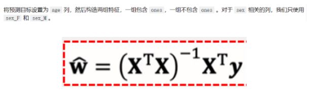
将鲍鱼数据集划分为训练集和测试集

#拆分训练集和测试集
from sklearn.model_selection import train_test_split

X_train,X_test,y_train,y_test = train_test_split(X,y,test_size=0.2,random_state=111)

	length	diameter	height	whole weight	shucked weight	viscera weight	shell weight	sex_F	sex_M	ones
0	0.455	0.365	0.095	0.5140	0.2245	0.1010	0.1500	0	1	1
1	0.350	0.265	0.090	0.2255	0.0995	0.0485	0.0700	0	1	1
2	0.530	0.420	0.135	0.6770	0.2565	0.1415	0.2100	1	0	1
3	0.440	0.365	0.125	0.5160	0.2155	0.1140	0.1550	0	1	1
4	0.330	0.255	0.080	0.2050	0.0895	0.0395	0.0550	0	0	1
5	0.425	0.300	0.095	0.3515	0.1410	0.0775	0.1200	0	0	1
6	0.530	0.415	0.150	0.7775	0.2370	0.1415	0.3300	1	0	1
7	0.545	0.425	0.125	0.7680	0.2940	0.1495	0.2600	1	0	1
8	0.475	0.370	0.125	0.5095	0.2165	0.1125	0.1650	0	1	1
9	0.550	0.440	0.150	0.8945	0.3145	0.1510	0.3200	1	0	1
10	0.525	0.380	0.140	0.6065	0.1940	0.1475	0.2100	1	0	1
11	0.430	0.350	0.110	0.4060	0.1675	0.0810	0.1350	0	1	1
12	0.490	0.380	0.135	0.5415	0.2175	0.0950	0.1900	0	1	1
13	0.535	0.405	0.145	0.6845	0.2725	0.1710	0.2050	1	0	1
14	0.470	0.355	0.100	0.4755	0.1675	0.0805	0.1850	1	0	1
15	0.500	0.400	0.130	0.6645	0.2580	0.1330	0.2400	0	1	1
16	0.355	0.280	0.085	0.2905	0.0950	0.0395	0.1150	0	0	1
17	0.440	0.340	0.100	0.4510	0.1880	0.0870	0.1300	1	0	1
18	0.365	0.295	0.080	0.2555	0.0970	0.0430	0.1000	0	1	1
19	0.450	0.320	0.100	0.3810	0.1705	0.0750	0.1150	0	1	1
20	0.355	0.280	0.095	0.2455	0.0955	0.0620	0.0750	0	1	1
21	0.380	0.275	0.100	0.2255	0.0800	0.0490	0.0850	0	0	1
22	0.565	0.440	0.155	0.9395	0.4275	0.2140	0.2700	1	0	1
23	0.550	0.415	0.135	0.7635	0.3180	0.2100	0.2000	1	0	1
24	0.615	0.480	0.165	1.1615	0.5130	0.3010	0.3050	1	0	1
25	0.560	0.440	0.140	0.9285	0.3825	0.1880	0.3000	1	0	1
26	0.580	0.450	0.185	0.9955	0.3945	0.2720	0.2850	1	0	1
27	0.590	0.445	0.140	0.9310	0.3560	0.2340	0.2800	0	1	1
28	0.605	0.475	0.180	0.9365	0.3940	0.2190	0.2950	0	1	1
29	0.575	0.425	0.140	0.8635	0.3930	0.2270	0.2000	0	1	1
...	...	...	...	...	...	...	...	...	...	...
4147	0.695	0.550	0.195	1.6645	0.7270	0.3600	0.4450	0	1	1
4148	0.770	0.605	0.175	2.0505	0.8005	0.5260	0.3550	0	1	1
4149	0.280	0.215	0.070	0.1240	0.0630	0.0215	0.0300	0	0	1
4150	0.330	0.230	0.080	0.1400	0.0565	0.0365	0.0460	0	0	1
4151	0.350	0.250	0.075	0.1695	0.0835	0.0355	0.0410	0	0	1
4152	0.370	0.280	0.090	0.2180	0.0995	0.0545	0.0615	0	0	1
4153	0.430	0.315	0.115	0.3840	0.1885	0.0715	0.1100	0	0	1
4154	0.435	0.330	0.095	0.3930	0.2190	0.0750	0.0885	0	0	1
4155	0.440	0.350	0.110	0.3805	0.1575	0.0895	0.1150	0	0	1
4156	0.475	0.370	0.110	0.4895	0.2185	0.1070	0.1460	0	1	1
4157	0.475	0.360	0.140	0.5135	0.2410	0.1045	0.1550	0	1	1
4158	0.480	0.355	0.110	0.4495	0.2010	0.0890	0.1400	0	0	1
4159	0.560	0.440	0.135	0.8025	0.3500	0.1615	0.2590	1	0	1
4160	0.585	0.475	0.165	1.0530	0.4580	0.2170	0.3000	1	0	1
4161	0.585	0.455	0.170	0.9945	0.4255	0.2630	0.2845	1	0	1
4162	0.385	0.255	0.100	0.3175	0.1370	0.0680	0.0920	0	1	1
4163	0.390	0.310	0.085	0.3440	0.1810	0.0695	0.0790	0	0	1
4164	0.390	0.290	0.100	0.2845	0.1255	0.0635	0.0810	0	0	1
4165	0.405	0.300	0.085	0.3035	0.1500	0.0505	0.0880	0	0	1
4166	0.475	0.365	0.115	0.4990	0.2320	0.0885	0.1560	0	0	1
4167	0.500	0.380	0.125	0.5770	0.2690	0.1265	0.1535	0	1	1
4168	0.515	0.400	0.125	0.6150	0.2865	0.1230	0.1765	1	0	1
4169	0.520	0.385	0.165	0.7910	0.3750	0.1800	0.1815	0	1	1
4170	0.550	0.430	0.130	0.8395	0.3155	0.1955	0.2405	0	1	1
4171	0.560	0.430	0.155	0.8675	0.4000	0.1720	0.2290	0	1	1
4172	0.565	0.450	0.165	0.8870	0.3700	0.2390	0.2490	1	0	1
4173	0.590	0.440	0.135	0.9660	0.4390	0.2145	0.2605	0	1	1
4174	0.600	0.475	0.205	1.1760	0.5255	0.2875	0.3080	0	1	1
4175	0.625	0.485	0.150	1.0945	0.5310	0.2610	0.2960	1	0	1
4176	0.710	0.555	0.195	1.9485	0.9455	0.3765	0.4950	0	1	1

4177 rows × 10 columns

实现线性回归和岭回归

使用numpy实现线性回归

import numpy as np

def linear_regression(X,y):
    w = np.zeros_like(X.shape[1])
    if np.linalg.det(X.T.dot(X)) != 0:
        w = np.linalg.inv(X.T.dot(X)).dot(X.T).dot(y)
    return w

#使用上述实现的线性回归模型在鲍鱼训练集上训练模型
w1 = linear_regression(X_train,y_train)

w1 = pd.DataFrame(data = w1,index=X.columns,columns =["numpy_w"])
w1.round(decimals=2)

	numpy_w
length	-1.12
diameter	10.00
height	20.74
whole weight	9.61
shucked weight	-20.05
viscera weight	-12.07
shell weight	6.55
sex_F	0.88
sex_M	0.87
ones	4.32

使用sklearn实现线性回归

from sklearn.linear_model import LinearRegression 
lr = LinearRegression()
lr.fit(X_train[features_without_ones],y_train)
print(lr.coef_)

[ -1.118146    10.00094599  20.73712616   9.61484657 -20.05079291
 -12.06849193   6.54529076   0.87855188   0.87283083]

w1

	numpy_w
length	-1.118146
diameter	10.000946
height	20.737126
whole weight	9.614847
shucked weight	-20.050793
viscera weight	-12.068492
shell weight	6.545291
sex_F	0.878552
sex_M	0.872831
ones	4.324477

w_lr=[]
w_lr.extend(lr.coef_)
w_lr.append(lr.intercept_)
w1["lr_sklearn_w"]=w_lr
w1.round(decimals=2)

	numpy_w	lr_sklearn_w
length	-1.12	-1.12
diameter	10.00	10.00
height	20.74	20.74
whole weight	9.61	9.61
shucked weight	-20.05	-20.05
viscera weight	-12.07	-12.07
shell weight	6.55	6.55
sex_F	0.88	0.88
sex_M	0.87	0.87
ones	4.32	4.32

#做正则化时不包含b lambda I不是真正的系数

使用Numpy实现岭回归

def ridge_regression(X,y,ridge_lambda):
    penalty_matrix = np.eye(X.shape[1])
    penalty_matrix[X.shape[1]-1][X.shape[1]-1] = 0
    w = np.linalg.inv(X.T.dot(X) + ridge_lambda * penalty_matrix).dot(X.T).dot(y)
    return w

在鲍鱼训练集上使用ridge_regression函数训练岭回归模型，正则化系数设置为1

w2 = ridge_regression(X_train,y_train,1.0)
print(w2)

[  2.30976528   6.72038628  10.23298909   7.05879189 -17.16249532
  -7.2343118    9.3936994    0.96869974   0.9422174    4.80583032]

w1["numpy_ridge_w"] = w2
w1.round(decimals=2)

	numpy_w	lr_sklearn_w	numpy_ridge_w
length	-1.12	-1.12	2.31
diameter	10.00	10.00	6.72
height	20.74	20.74	10.23
whole weight	9.61	9.61	7.06
shucked weight	-20.05	-20.05	-17.16
viscera weight	-12.07	-12.07	-7.23
shell weight	6.55	6.55	9.39
sex_F	0.88	0.88	0.97
sex_M	0.87	0.87	0.94
ones	4.32	4.32	4.81

利用sklearn实现岭回归

与sklearn中岭回归对比，同样正则化叙述设置为1

from sklearn.linear_model import Ridge
ridge = Ridge(alpha=1.0)
ridge.fit(X_train[features_without_ones],y_train)
w_ridge = []
w_ridge.extend(ridge.coef_)
w_ridge.append(ridge.intercept_)
w1["ridge_sklearn_w"] = w_ridge
w1.round(decimals=2)

	numpy_w	lr_sklearn_w	numpy_ridge_w	ridge_sklearn_w
length	-1.12	-1.12	2.31	2.31
diameter	10.00	10.00	6.72	6.72
height	20.74	20.74	10.23	10.23
whole weight	9.61	9.61	7.06	7.06
shucked weight	-20.05	-20.05	-17.16	-17.16
viscera weight	-12.07	-12.07	-7.23	-7.23
shell weight	6.55	6.55	9.39	9.39
sex_F	0.88	0.88	0.97	0.97
sex_M	0.87	0.87	0.94	0.94
ones	4.32	4.32	4.81	4.81

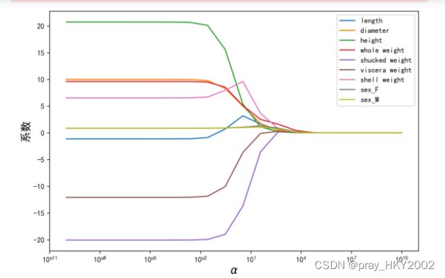
岭迹分析

alphas = np.logspace(-10,10,20)
coef = pd.DataFrame()
for alpha in alphas:
    ridge_clf = Ridge(alpha=alpha)
    ridge_clf.fit(X_train[features_without_ones],y_train)
    df = pd.DataFrame([ridge_clf.coef_],columns=X_train[features_without_ones].columns)
    df['alpha']=alpha
    coef =coef.append(df,ignore_index=True)
coef.round(decimals=2)

	length	diameter	height	whole weight	shucked weight	viscera weight	shell weight	sex_F	sex_M	alpha
0	-1.12	10.00	20.74	9.61	-20.05	-12.07	6.55	0.88	0.87	0.000000e+00
1	-1.12	10.00	20.74	9.61	-20.05	-12.07	6.55	0.88	0.87	0.000000e+00
2	-1.12	10.00	20.74	9.61	-20.05	-12.07	6.55	0.88	0.87	0.000000e+00
3	-1.12	10.00	20.74	9.61	-20.05	-12.07	6.55	0.88	0.87	0.000000e+00
4	-1.12	10.00	20.74	9.61	-20.05	-12.07	6.55	0.88	0.87	0.000000e+00
5	-1.12	10.00	20.74	9.61	-20.05	-12.07	6.55	0.88	0.87	0.000000e+00
6	-1.12	10.00	20.73	9.61	-20.05	-12.07	6.55	0.88	0.87	0.000000e+00
7	-1.10	9.98	20.68	9.60	-20.04	-12.05	6.56	0.88	0.87	0.000000e+00
8	-0.88	9.79	20.13	9.50	-19.94	-11.86	6.71	0.88	0.88	3.000000e-02
9	0.73	8.33	15.60	8.55	-18.97	-10.05	7.98	0.92	0.90	3.000000e-01
10	3.20	5.02	5.40	5.11	-13.71	-3.67	9.61	1.07	1.00	3.360000e+00
11	1.66	1.76	1.12	2.53	-3.54	-0.09	3.67	1.33	1.11	3.793000e+01
12	0.51	0.47	0.22	1.63	0.18	0.30	0.79	0.89	0.69	4.281300e+02
13	0.12	0.10	0.04	0.46	0.15	0.09	0.16	0.21	0.16	4.832930e+03
14	0.01	0.01	0.00	0.05	0.02	0.01	0.02	0.02	0.02	5.455595e+04
15	0.00	0.00	0.00	0.00	0.00	0.00	0.00	0.00	0.00	6.158482e+05
16	0.00	0.00	0.00	0.00	0.00	0.00	0.00	0.00	0.00	6.951928e+06
17	0.00	0.00	0.00	0.00	0.00	0.00	0.00	0.00	0.00	7.847600e+07
18	0.00	0.00	0.00	0.00	0.00	0.00	0.00	0.00	0.00	8.858668e+08
19	0.00	0.00	0.00	0.00	0.00	0.00	0.00	0.00	0.00	1.000000e+10

plt.rcParams['figure.dpi'] = 300#分辨率
plt.figure(figsize=(9,6))
coef['alpha']=coef['alpha']

for feature in X_train.columns[:-1]:
    plt.plot('alpha',feature,data=coef)
ax = plt.gca()
ax.set_xscale('log')
plt.legend(loc='upper right')
plt.xlabel(r'$\alpha$',fontsize=15)
plt.ylabel('系数',fontsize=15)

Text(0, 0.5, '系数')



Font 'default' does not have a glyph for '-' [U+2212], substituting with a dummy symbol.
Font 'default' does not have a glyph for '-' [U+2212], substituting with a dummy symbol.
Font 'default' does not have a glyph for '-' [U+2212], substituting with a dummy symbol.
Font 'default' does not have a glyph for '-' [U+2212], substituting with a dummy symbol.
Font 'default' does not have a glyph for '-' [U+2212], substituting with a dummy symbol.
Font 'default' does not have a glyph for '-' [U+2212], substituting with a dummy symbol.
Font 'default' does not have a glyph for '-' [U+2212], substituting with a dummy symbol.
Font 'default' does not have a glyph for '-' [U+2212], substituting with a dummy symbol.
Font 'default' does not have a glyph for '-' [U+2212], substituting with a dummy symbol.
Font 'default' does not have a glyph for '-' [U+2212], substituting with a dummy symbol.
Font 'default' does not have a glyph for '-' [U+2212], substituting with a dummy symbol.
Font 'default' does not have a glyph for '-' [U+2212], substituting with a dummy symbol.
Font 'default' does not have a glyph for '-' [U+2212], substituting with a dummy symbol.
Font 'default' does not have a glyph for '-' [U+2212], substituting with a dummy symbol.
Font 'default' does not have a glyph for '-' [U+2212], substituting with a dummy symbol.
Font 'default' does not have a glyph for '-' [U+2212], substituting with a dummy symbol.

使用LASSO构建鲍鱼年龄预测模型

from sklearn.linear_model import Lasso
lasso = Lasso(alpha=0.01)
lasso.fit(X_train[features_without_ones],y_train)
print(lasso.coef_)
print(lasso.intercept_)

[  0.           6.37435514   0.           4.46703234 -13.44947667
  -0.          11.85934842   0.98908791   0.93313403]
6.500338023591298

LASSO的正则化路径

coef = pd.DataFrame()
for alpha in np.linspace(0.0001,0.2,20):
    lasso_clf = Lasso(alpha=alpha)
    lasso_clf.fit(X_train[features_without_ones],y_train)
    df = pd.DataFrame([lasso_clf.coef_],columns=X_train[features_without_ones].columns)
    df['alpha']=alpha
    coef = coef.append(df,ignore_index=True)
coef.head()
#绘图
plt.figure(figsize=(9,6),dpi=600)
for feature in X_train.columns[:-1]:
    plt.plot('alpha',feature,data=coef)
plt.legend(loc='upper right')
plt.xlabel(r'$\alpha$',fontsize=15)
plt.ylabel('系数',fontsize=15)
plt.show()

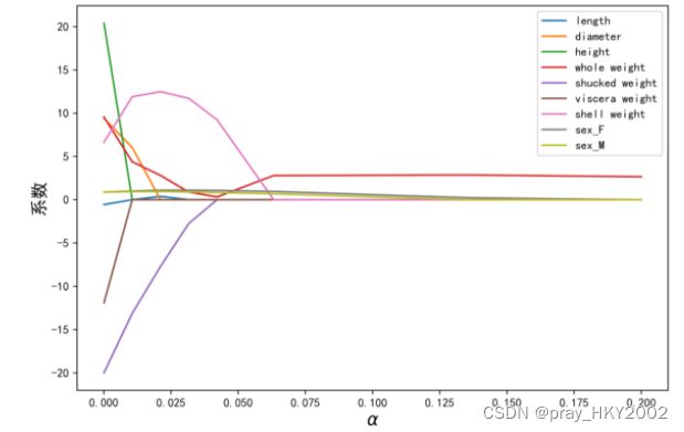
coef

	length	diameter	height	whole weight	shucked weight	viscera weight	shell weight	sex_F	sex_M	alpha
0	-0.568043	9.39275	20.390041	9.542038	-19.995972	-11.900326	6.635352	0.881496	0.875132	0.000100
1	0.000000	6.02573	0.000000	4.375754	-13.127223	-0.000000	11.897189	0.995137	0.934129	0.010621
2	0.384927	0.00000	0.000000	2.797815	-7.702209	-0.000000	12.478541	1.093479	0.948281	0.021142
3	0.000000	0.00000	0.000000	0.884778	-2.749504	0.000000	11.705974	1.098990	0.897673	0.031663
4	0.000000	0.00000	0.000000	0.322742	-0.000000	0.000000	9.225919	1.072991	0.834021	0.042184
5	0.000000	0.00000	0.000000	1.555502	-0.000000	0.000000	4.610425	1.013824	0.757891	0.052705
6	0.000000	0.00000	0.000000	2.786784	-0.000000	0.000000	0.000000	0.954710	0.681821	0.063226
7	0.000000	0.00000	0.000000	2.797514	-0.000000	0.000000	0.000000	0.848412	0.581613	0.073747
8	0.000000	0.00000	0.000000	2.807843	-0.000000	0.000000	0.000000	0.742529	0.481711	0.084268
9	0.000000	0.00000	0.000000	2.818184	-0.000000	0.000000	0.000000	0.636632	0.381799	0.094789
10	0.000000	0.00000	0.000000	2.828630	-0.000000	0.000000	0.000000	0.530615	0.281801	0.105311
11	0.000000	0.00000	0.000000	2.838944	-0.000000	0.000000	0.000000	0.424750	0.181912	0.115832
12	0.000000	0.00000	0.000000	2.849325	-0.000000	0.000000	0.000000	0.318807	0.081967	0.126353
13	0.000000	0.00000	0.000000	2.851851	-0.000000	0.000000	0.000000	0.225024	0.000000	0.136874
14	0.000000	0.00000	0.000000	2.819079	-0.000000	0.000000	0.000000	0.186157	0.000000	0.147395
15	0.000000	0.00000	0.000000	2.786307	-0.000000	0.000000	0.000000	0.147290	0.000000	0.157916
16	0.000000	0.00000	0.000000	2.753535	0.000000	0.000000	0.000000	0.108422	0.000000	0.168437
17	0.000000	0.00000	0.000000	2.720762	0.000000	0.000000	0.000000	0.069555	0.000000	0.178958
18	0.000000	0.00000	0.000000	2.687990	0.000000	0.000000	0.000000	0.030688	0.000000	0.189479
19	0.000000	0.00000	0.000000	2.652940	0.000000	0.000000	0.000000	0.000000	0.000000	0.200000

from sklearn.metrics import mean_squared_error
from sklearn.metrics import mean_absolute_error
from sklearn.metrics import r2_score

#MAE
y_test_pred_lr = lr.predict(X_test.iloc[:,:-1])
print(round(mean_absolute_error(y_test,y_test_pred_lr),4))

1.6016

y_test_pred_ridge = ridge.predict(X_test[features_without_ones])
print(round(mean_absolute_error(y_test,y_test_pred_ridge),4))

1.5984

y_test_pred_lasso = lasso.predict(X_test[features_without_ones])
print(round(mean_absolute_error(y_test,y_test_pred_lasso),4))

1.6402

#MSE
y_test_pred_lr = lr.predict(X_test.iloc[:,:-1])
print(round(mean_squared_error(y_test,y_test_pred_lr),4))

5.3009

y_test_pred_ridge = ridge.predict(X_test[features_without_ones])
print(round(mean_squared_error(y_test,y_test_pred_ridge),4))

4.959

y_test_pred_lasso = lasso.predict(X_test[features_without_ones])
print(round(mean_squared_error(y_test,y_test_pred_lasso),4))

5.1

#R2系数
print(round(r2_score(y_test,y_test_pred_lr),4))
print(round(r2_score(y_test,y_test_pred_ridge),4))
print(round(r2_score(y_test,y_test_pred_lasso),4))

0.5257
0.5563
0.5437

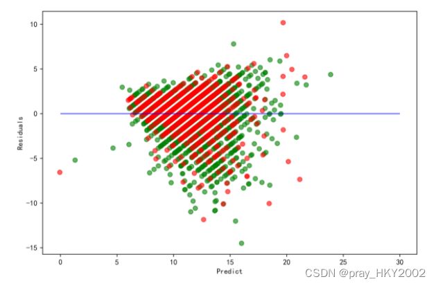
残差图

plt.figure(figsize=(9,6),dpi=600)
y_train_pred_ridge = ridge.predict(X_train[features_without_ones])
plt.scatter(y_train_pred_ridge,y_train_pred_ridge - y_train,c="g",alpha=0.6)
plt.scatter(y_test_pred_ridge,y_test_pred_ridge - y_test,c="r",alpha=0.6)
plt.hlines(y=0,xmin=0,xmax=30,color="b",alpha=0.6)
plt.ylabel("Residuals")
plt.xlabel("Predict")

Text(0.5, 0, 'Predict')

你可能感兴趣的:(python,机器学习,数据挖掘,逻辑回归)

Numpy布尔索引与掩码新缸中之脑 Numpy
NumPy是用于科学计算和处理多维数组数据的最流行的Python库之一。NumPy提供了强大的功能，可以根据布尔条件从数组中索引和提取元素，这称为布尔索引或掩码。掌握布尔索引和掩码可以使用NumPy进行高效的数据操作和分析。本综合指南将解释你需要了解的有关NumPy中布尔索引和掩码的所有信息，包括关键概念、用法和示例，以帮助你在自己的项目中利用这些技术。NSDT工具推荐：Three.jsAI纹理开
python 数据挖掘与机器学习科研的力量人工智能 ChatGPT python 数据挖掘机器学习神经网络随机森林决策树贝叶斯
近年来，Python编程语言受到越来越多科研人员的喜爱，在多个编程语言排行榜中持续夺冠。同时，伴随着深度学习的快速发展，人工智能技术在各个领域中的应用越来越广泛。机器学习是人工智能的基础，因此，掌握常用机器学习算法的工作原理，并能够熟练运用Python建立实际的机器学习模型，是开展人工智能相关研究的前提和基础。模块一：课前准备Python编程基础与进阶Python编程入门1、Python环境搭建（
Python+pytest+jenkins 多插件 pdf电子书目录 weixin_43946945 python pytest jenkins pdf
第1章pytest入门11.1资源获取41.2运行Pytest51.3运行单个测试用例101.4使用命令行选项10--collect-only选项11-k选项11-m选项12-x选项13--maxfail＝num15-s与--capture＝method16-lf（--lastfailed）选项16--ff（--failed-first）选项17-v（--verbose）选项17-q（--quie
python金融实战教程pdf 目录 weixin_43946945 python 金融 pdf 经验分享全文检索学习
python金融实战教程pdf目录:http://literalink.top/resource/detail/7186336410574524416第1章Python简介及安装11.1Python简介11.2如何安装Python31.3Python的不同版本31.4运行Python的3种方式41.4.1用GUI启动Python41.4.2从Python命令行启动Python51.4.3从DOS窗
能下载各类书籍的pdf电子书网站 weixin_43946945 pdf python 经验分享
能下载各类书籍的pdf电子书网站最近我又在学习pythonui自动化了，以前刚接触python那时候只会用我要自学网，还挺好用的，助我学完了python基础。但是现在需要更深入的学习，自学网已经不能满足我了，因此我翻遍咸鱼，5块钱买了一份资料，结果收到后打开是python2的，我需要的是python3…算了，还是继续网上找吧。我就找啊找，功夫不负有心人，我不仅找到了我需要的专业方面的书籍，我还发现
python数据类型与常用使用函数卑微的辣椒 python 开发语言
试着对python的数据类型进行了整理，之前浅浅的学习了python，总感觉自己学习的很表面，给个python的题也不能很快的想到怎么去解，感觉还是的从基础开始在渗透下。下面是我整理的python的数据类型及常用的一些函数。一、Python的数据类型1.整型int是Python中表示整数的数据类型。它可以是正数、负数或零。2.字符串string是Python中表示文本字符串的数据类型。它由一系列字
python如何控制手机发短信_利用Python实现手机短信监控通知 weixin_39644021 python如何控制手机发短信
日常运维工作中，通常是邮件报警机制，但邮件可能不被及时查看，导致问题出现得不到及时有效处理。所以想到用Python实现发短信功能，当监控到问题出现时，短信报警，使问题能得到及时的处理。当然，我相信，用Python发短信应用场景不止此一处，下面我们开始Python发短信的实现。首先，看下成果展示：然后，看下代码实现：是不是非常简单！现在开始具体讲解，如何实现Python发短信功能。操作步骤1、安装模
使用python实现往手机发短信（基于twilio） weixin_33953249
#导包导入twilio客户端fromtwilio.restimportClient#定义短信sidaccount_sid='AC7fcb4e7e65f2113b320f1bc280fe7c32'#定义秘钥auth_token='f35022077f53f356f0469a43ffa28c9f'#定义客户端对象clinet=Client(account_sid,auth_token)#定义短信内容第
C语言入门基础知识（持续更新中）社恐小美~ C语言 c语言开发语言汇编
1.1什么是C语言1.1.1计算机语言------语言是人与人之间交流媒介计算机语言的发展历程------机器语言->汇编语言->高级语言(1.面向过程：C2.面向对象：C++，JAVA,python,PHP······)1.1.2机器语言机器语言：计算机是一种电子设备，计算机处理的数字信号是0和1去记录相应信息，利用数字语言0和1来表示计算机能够识别的通断和断电两种状态。那么计算机的语言成为机器
1区9+非肿瘤纯生信，逻辑清晰易懂，机器学习筛选关键基因的纯生信也可以发高水平期刊，抓紧上车！生信小课堂
影响因子：9.186关于非肿瘤生信，我们也解读过很多，主要有以下类型1单个疾病WGCNA+PPI分析筛选hub基因。2单个疾病结合免疫浸润，热点基因集，机器学习算法等。3两种相关疾病联合分析，包括非肿瘤结合非肿瘤，非肿瘤结合肿瘤或者非肿瘤结合泛癌分析4基于分型的非肿瘤生信分析5单细胞结合普通转录组生信分析目前非肿瘤生信发文的门槛较低，有需要的朋友欢迎交流研究概述：本研究首先使用R语言在三个基因表达
网络自动化新篇章：Ansible与Python的强强联合姬如雅Brina
网络自动化新篇章：Ansible与Python的强强联合在这个数字化和自动化的时代，网络管理已经不再局限于手动配置和管理。开源项目“NetworkAutomationwithAnsibleandPython”将带你进入一个全新的世界，通过强大的工具和语言实现网络设备的高效管理和自动化部署。让我们一起探索这个令人兴奋的项目。项目介绍该项目源于InterOpVegas2015的演讲材料，由网络自动化专
网络自动化：利用Python和Ansible实现网络配置管理 hai40587 网络自动化 python
网络自动化：利用Python和Ansible实现网络配置管理在当今快速变化的IT环境中，网络自动化已成为提升运维效率、减少人为错误、加速服务交付的关键技术之一。Python和Ansible作为两种强大的工具，在网络配置管理中发挥着重要作用。本文将深入探讨如何利用Python和Ansible实现网络自动化，包括它们的基本概念、优势、应用场景、实施步骤以及最佳实践。一、引言网络配置管理是指对网络设备进
kafka系列之：使用python消费kafka Topic数据快乐骑行^_^ 大数据 kafka系列 python
kafka系列之：使用python消费kafkaTopic数据一、创建kafkaConsumer三、查看分区四、查看分区信息五、查看当前消费的Topic六、获取当前消费者可消费的偏移量七、获取当前Topic最大的偏移量八、获取当前kafkatopic、分区和分区偏移量九、重置偏移量十、根据重置的偏移量消费数据十一、使用python消费kafkaTopic数据完整详细注释代码一、创建kafkaCon
python对象的引用和可变性百流 python笔记 python
Python对象的引用和可变性1.变量是标签当一个对象被绑定到一个变量上后，如果再将该变量绑定到另一个对象上，之前的引用不会受到影响>>>a=[1,2,3]>>>b=a>>>a.append(4)>>>b[1,2,3,4]变量a,b引用同一个列表而不是创建新的副本创建对象之后才会把变量分配给对象>>>classGizmo:...def__init__(self):...print('Gizmoid
python中func自定义函数_Python函数之自定义函数&作用域&闭包瞄小七.sunshine
一前言1.1为什么要用函数代码的组织结构更清晰，可读性好；遇到重复的功能不需要重新编写代码，调用函数即可，代码不会冗余；功能需要扩展时，只需要修改函数内容即可，实现统一管理，降低代码维护难度函数式编程最重要的是增强代码的重用性和可读性1.2函数是什么想象生活中的例子，修理工需要事先准备好工具箱里面放好锤子，扳手，钳子等工具，然后遇到锤钉子的场景，拿来锤子用就可以，而无需临时再制造一把锤子。修理工-
使用python创建kafka的topic 百流 python笔记 python kafka 开发语言
文章目录使用python创建kafka的topickafka基本概念所需安装的包代码样例使用python创建kafka的topickafka基本概念Apache‌Kafka是一个开源的分布式流处理平台，设计用于处理实时数据流。它由‌Apache软件基金会开发，使用‌Scala和‌Java编写。‌#特性1.‌分布式‌：Kafka是分布式的系统，支持多分区和多副本，确保了数据的可靠性和系统的可扩展性。
AI中的核心概念解读：深度学习、机器学习、神经网络与自然语言处理 wypdao 人工智能 AIGC 算法人工智能深度学习机器学习
人工智能（AI）是一个涵盖广泛领域的技术词汇，近年来受到了越来越多的关注和应用。然而，对于刚接触AI的初学者或非专业人士来说，理解其中的核心概念，特别是深度学习、机器学习、神经网络与自然语言处理之间的区别，可能显得有些复杂。本文将帮助读者梳理这些重要概念，厘清它们之间的关系和区别。一、人工智能（AI）首先，人工智能（AI）是一个广泛的领域，包含了任何通过计算机程序实现的智能行为。AI的目标是让机器
机器学习：svm算法原理的优缺点和适应场景夜清寒风支持向量机算法机器学习
1、概述：基本原理：间隔（Margin）：SVM试图找到一个超平面，这个超平面不仅能够区分不同的类别，而且具有最大的间隔。间隔是数据点到超平面的最近距离。支持向量（SupportVectors）：这些是距离超平面最近的数据点，它们决定了超平面的位置和方向。支持向量机（SVM）是一种在机器学习领域广泛使用的监督学习模型，它通过找到数据点之间的最优超平面来进行分类或回归分析。以下是SVM算法的一些优缺
昇思25天学习打卡十分钟ll 昇思25天学习打卡 python pytorch 视觉检测图像处理
@[TOC]《昇思25天学习打卡营第02天|lulul》张量Tensor张量tensor是在机器学习和深度学习中广泛应用的数据概念，张量是多维数组的泛化，能够表示标量（0维张量）、向量（1维张量）、矩阵（2维张量）及更高维的数组。张量基本用法（mindspore）data=[1,0,1,0]x_data=Tensor(data)print(x_data,x_data.shape,x_data.dt
基于yolov8的脑肿瘤检测系统python源码+onnx模型+评估指标曲线+精美GUI界面 FL1623863129 深度学习 YOLO 人工智能
【算法介绍】基于YOLOv8的脑肿瘤检测系统是一项前沿的医疗应用，该系统利用YOLOv8这一高效的目标检测算法，实现对脑肿瘤病灶的快速、准确识别。YOLOv8作为YOLO系列的最新版本，不仅继承了前代版本在速度和精度上的优势，还通过改进的网络结构和优化策略，进一步提升了模型性能。在脑肿瘤检测中，YOLOv8通过深度学习技术，自动从脑部图像中提取特征，并学习目标的特征表示和位置信息。系统采用模块化设
如何使用python抓包，附代码 Uncle 城 python 网络开发语言 AI
以下为您介绍多种使用Python进行抓包的方法及代码示例：使用Scapy库进行抓包：首先确保已经安装了Scapy库。如果没有安装，可以使用以下命令安装：pipinstallscapy。创建一个名为packet_sniffer.py的Python文件，并输入以下代码：fromscapy.allimport*defpacket_callback(packet):print(packet.summary
[2020]tensorflow2.1-GPU + CUDA +CUDNN配置过程记录夏迪End
最近几天做视频数据集的时候要用到tensorflow2的gpu训练版本，要安装对应版本的cuda和cudnn，网上的教程五花八门，我尝试了很多论坛的方法，有些能用有些不可以（也可能是我操作错误），经过两天调试终于能够运行了。1介绍使用的版本：Win10，python3.7，tensorflow2.1-GPU，CUDA10.1,CUDNN7.6.5，显卡驱动版本是425.31（用的IDE是pycha
【Python机器学习】NLP词频背后的含义——隐性语义分析 zhangbin_237 Python机器学习 python 机器学习自然语言处理人工智能开发语言
隐性语义分析基于最古老和最常用的降维技术——奇异值分解（SVD）。SVD将一个矩阵分解成3个方阵，其中一个是对角矩阵。SVD的一个应用是求逆矩阵。一个矩阵可以分解成3个最简单的方阵，然后对这些方阵求转置后再把它们相乘，就得到了原始矩阵的逆矩阵。它为我们提供了一个对大型复杂矩阵求逆的捷径。SVD适用于桁架结构的应力和应变分析等机械工程问题，它对电气工程中的电路分析也很有用，它甚至在数据科学中被用于基
Python编码—掌握Python与Kubernetes：构建高效微服务架构学步_技术 Python编码架构 python kubernetes
欢迎来到我的技术小筑，一个专为技术探索者打造的交流空间。在这里，我们不仅分享代码的智慧，还探讨技术的深度与广度。无论您是资深开发者还是技术新手，这里都有一片属于您的天空。让我们在知识的海洋中一起航行，共同成长，探索技术的无限可能。探索专栏：学步_技术的首页——持续学习，不断进步，让学习成为我们共同的习惯，让总结成为我们前进的动力。技术导航：人工智能：深入探讨人工智能领域核心技术。自动驾驶：分享自动
统计机器学习第十三章极大似然估计的性质——图解MLE的渐进正态性 cui_hao_nan 统计机器学习导论机器学习
n=10;t=10000;s=1/12/n;x=linspace(-0.4,0.4,100);y=1/sqrt(2*pi*s)*exp(-x.^2/(2*s));z=mean(rand(t,n)-0.5,2);figure(1);clf;holdonb=20;hist(z,b);h=plot(x,y*t/b*(max(z)-min(z)),'r-');这段代码的功能是生成随机数并进行直方图和曲线的
sqllabs游戏 Vanilla-li web安全
文章目录总体思路：less-1:less-2:less-3:less-4:less-5:less-6:less-7:less-8:布尔盲注less-9:时间盲注less-21:less-24:总体思路：1、第一件事情逃脱出单引号的控制闭合单引号2、单双引号需要成对出现在pythonphpJava中3、2个办法继续把多出来的单引号闭合，要么注释掉单引号4、MySQL注释符–#/***/*/url会编
动手学深度学习（pytorch）学习记录21-读写文件(模型与参数)[学习记录] walfar pytorch 深度学习 pytorch 学习
目录加载和保存张量加载和保存模型参数保存模型的好处众多，涵盖了从开发到部署的整个机器学习生命周期。节省资源：训练模型可能需要大量的时间和计算资源。保存模型可以避免重复训练，从而节省时间和计算资源。快速部署：一旦模型被训练并保存，它可以迅速部署到生产环境中，加速产品上市时间。版本控制：保存不同版本的模型有助于跟踪模型的迭代过程，便于比较和回滚到之前的版本。离线使用：保存的模型可以在没有网络连接的情况
python \uxx字符串转中文 hzw0510 python进阶 python 前端 javascript
python\uxx字符串转中文#假设我们有一个Unicode编码的字符串unicode_string="\\u4e2d\\u6587"#使用str()函数将Unicode编码转换为中文chinese_characters=str(unicode_string.encode('utf-8').decode('unicode_escape'
PyTorch 基础学习（14）- 归一化花千树-010 PyTorch pytorch 学习人工智能
系列文章：《PyTorch基础学习》文章索引概述归一化是数据预处理中的重要步骤之一，它可以将数据调整到特定的范围或分布，有助于加速训练并提高模型的性能。在机器学习中，不同的归一化方法适用于不同的场景。本文将详细介绍scikit-learn中的常见归一化方法及其应用。1.Min-Max归一化MinMaxScalerMin-Max归一化将数据缩放到指定范围，通常是[0,1]。这种方法保留了数据的相对关
windows11 上安装了python的wxpython模块，vscode运行时还是报错的解决方法 winfredzhang python vscode wxpython 解决问题
遇到问题：windows11上明明安装了python的wxpython模块，vscode运行时还是报错“Traceback(mostrecentcalllast):File“c:\pythoncode\new\tonguedetect.py”,line1,inimportwxModuleNotFoundError:Nomodulenamed‘wx’”如何解决？看起来你已经安装了wxPython模块
LeetCode[位运算] - #137 Single Number II Cwind java Algorithm LeetCode 题解位运算
原题链接：#137 Single Number II 要求：给定一个整型数组，其中除了一个元素之外，每个元素都出现三次。找出这个元素注意：算法的时间复杂度应为O(n)，最好不使用额外的内存空间难度：中等分析：与#136类似，都是考察位运算。不过出现两次的可以使用异或运算的特性 n XOR n = 0, n XOR 0 = n，即某一
《JavaScript语言精粹》笔记 aijuans JavaScript
0、JavaScript的简单数据类型包括数字、字符创、布尔值（true/false）、null和undefined值，其它值都是对象。 1、JavaScript只有一个数字类型，它在内部被表示为64位的浮点数。没有分离出整数，所以1和1.0的值相同。 2、NaN是一个数值，表示一个不能产生正常结果的运算结果。NaN不等于任何值，包括它本身。可以用函数isNaN(number)检测NaN,但是
你应该更新的Java知识之常用程序库 Kai_Ge java
在很多人眼中，Java 已经是一门垂垂老矣的语言，但并不妨碍 Java 世界依然在前进。如果你曾离开 Java，云游于其它世界，或是每日只在遗留代码中挣扎，或许是时候抬起头，看看老 Java 中的新东西。 Guava Guava[gwɑ:və]，一句话，只要你做Java项目，就应该用Guava（Github）。 guava 是 Google 出品的一套 Java 核心库，在我看来，它甚至应该
HttpClient 120153216 httpclient
/** * 可以传对象的请求转发，对象已流形式放入HTTP中 */ public static Object doPost(Map<String,Object> parmMap,String url) { Object object = null; HttpClient hc = new HttpClient(); String fullURL
Django model字段类型清单 2002wmj django
Django 通过 models 实现数据库的创建、修改、删除等操作，本文为模型中一般常用的类型的清单，便于查询和使用： AutoField：一个自动递增的整型字段，添加记录时它会自动增长。你通常不需要直接使用这个字段；如果你不指定主键的话，系统会自动添加一个主键字段到你的model。(参阅自动主键字段) BooleanField：布尔字段,管理工具里会自动将其描述为checkbox。 Cha
在SQLSERVER中查找消耗CPU最多的SQL 357029540 SQL Server
返回消耗CPU数目最多的10条语句 SELECT TOP 10 total_worker_time/execution_count AS avg_cpu_cost, plan_handle, execution_count, (SELECT SUBSTRING(text, statement_start_of
Myeclipse项目无法部署，Undefined exploded archive location 7454103 eclipse MyEclipse
做个备忘！错误信息为： Undefined exploded archive location 原因：在工程转移过程中，导致工程的配置文件出错；解决方法：
GMT时间格式转换 adminjun GMT 时间转换
普通的时间转换问题我这里就不再罗嗦了，我想大家应该都会那种低级的转换问题吧，现在我向大家总结一下如何转换GMT时间格式，这种格式的转换方法网上还不是很多，所以有必要总结一下，也算给有需要的朋友一个小小的帮助啦。 1、可以使用 SimpleDateFormat SimpleDateFormat EEE-三位星期 d-天 MMM-月 yyyy-四位年
Oracle数据库新装连接串问题 aijuans oracle数据库
割接新装了数据库，客户端登陆无问题，apache/cgi-bin程序有问题，sqlnet.log日志如下： Fatal NI connect error 12170. VERSION INFORMATION: TNS for Linux: Version 10.2.0.4.0 - Product
回顾java数组复制 ayaoxinchao java 数组
在写这篇文章之前，也看了一些别人写的，基本上都是大同小异。文章是对java数组复制基础知识的回顾，算是作为学习笔记，供以后自己翻阅。首先，简单想一下这个问题：为什么要复制数组？我的个人理解：在我们在利用一个数组时，在每一次使用，我们都希望它的值是初始值。这时我们就要对数组进行复制，以达到原始数组值的安全性。java数组复制大致分为3种方式：①for循环方式 ②clone方式 ③arrayCopy方
java web会话监听并使用spring注入 bewithme Java Web
在java web应用中，当你想在建立会话或移除会话时，让系统做某些事情，比如说，统计在线用户，每当有用户登录时，或退出时，那么可以用下面这个监听器来监听。 import java.util.ArrayList; import java.ut
NoSQL数据库之Redis数据库管理(Redis的常用命令及高级应用) bijian1013 redis 数据库 NoSQL
一 .Redis常用命令 Redis提供了丰富的命令对数据库和各种数据库类型进行操作，这些命令可以在Linux终端使用。 a.键值相关命令 b.服务器相关命令 1.键值相关命令 &
java枚举序列化问题 bingyingao java 枚举序列化
对象在网络中传输离不开序列化和反序列化。而如果序列化的对象中有枚举值就要特别注意一些发布兼容问题: 1.加一个枚举值新机器代码读分布式缓存中老对象，没有问题，不会抛异常。老机器代码读分布式缓存中新对像，反序列化会中断，所以在所有机器发布完成之前要避免出现新对象，或者提前让老机器拥有新增枚举的jar。 2.删一个枚举值新机器代码读分布式缓存中老对象，反序列
【Spark七十八】Spark Kyro序列化 bit1129 spark
当使用SparkContext的saveAsObjectFile方法将对象序列化到文件，以及通过objectFile方法将对象从文件反序列出来的时候，Spark默认使用Java的序列化以及反序列化机制，通常情况下，这种序列化机制是很低效的，Spark支持使用Kyro作为对象的序列化和反序列化机制，序列化的速度比java更快，但是使用Kyro时要注意，Kyro目前还是有些bug。 Spark
Hybridizing OO and Functional Design bookjovi erlang haskell
推荐博文： Tell Above, and Ask Below - Hybridizing OO and Functional Design 文章中把OO和FP讲的深入透彻，里面把smalltalk和haskell作为典型的两种编程范式代表语言，此点本人极为同意，smalltalk可以说是最能体现OO设计的面向对象语言，smalltalk的作者Alan kay也是OO的最早先驱，
Java-Collections Framework学习与总结-HashMap BrokenDreams Collections
开发中常常会用到这样一种数据结构，根据一个关键字，找到所需的信息。这个过程有点像查字典，拿到一个key，去字典表中查找对应的value。Java1.0版本提供了这样的类java.util.Dictionary(抽象类)，基本上支持字典表的操作。后来引入了Map接口，更好的描述的这种数据结构。 &nb
读《研磨设计模式》-代码笔记-职责链模式-Chain Of Responsibility bylijinnan java 设计模式
声明：本文只为方便我个人查阅和理解，详细的分析以及源代码请移步原作者的博客http://chjavach.iteye.com/ /** * 业务逻辑：项目经理只能处理500以下的费用申请，部门经理是1000，总经理不设限。简单起见，只同意“Tom”的申请 * bylijinnan */ abstract class Handler { /*
Android中启动外部程序 cherishLC android
1、启动外部程序引用自： http://blog.csdn.net/linxcool/article/details/7692374 //方法一 Intent intent=new Intent(); //包名包名+类名（全路径） intent.setClassName("com.linxcool", "com.linxcool.PlaneActi
summary_keep_rate coollyj SUM
BEGIN /*DECLARE minDate varchar(20) ; DECLARE maxDate varchar(20) ;*/ DECLARE stkDate varchar(20) ; DECLARE done int default -1; /* 游标中注册服务器地址 */ DE
hadoop hdfs 添加数据目录出错 daizj hadoop hdfs 扩容
由于原来配置的hadoop data目录快要用满了，故准备修改配置文件增加数据目录，以便扩容，但由于疏忽，把core-site.xml, hdfs-site.xml配置文件dfs.datanode.data.dir 配置项增加了配置目录，但未创建实际目录，重启datanode服务时，报如下错误： 2014-11-18 08:51:39,128 WARN org.apache.hadoop.h
grep 目录级联查找 dongwei_6688 grep
在Mac或者Linux下使用grep进行文件内容查找时，如果给定的目标搜索路径是当前目录，那么它默认只搜索当前目录下的文件，而不会搜索其下面子目录中的文件内容，如果想级联搜索下级目录，需要使用一个“-r”参数： grep -n -r "GET" . 上面的命令将会找出当前目录“.”及当前目录中所有下级目录
yii 修改模块使用的布局文件 dcj3sjt126com yii layouts
方法一：yii模块默认使用系统当前的主题布局文件，如果在主配置文件中配置了主题比如: 'theme'=>'mythm', 那么yii的模块就使用 protected/themes/mythm/views/layouts 下的布局文件；如果未配置主题，那么 yii的模块就使用 protected/views/layouts 下的布局文件，总之默认不是使用自身目录 pr
设计模式之单例模式 come_for_dream 设计模式单例模式懒汉式饿汉式双重检验锁失败无序写入
今天该来的面试还没来，这个店估计不会来电话了，安静下来写写博客也不错，没事翻了翻小易哥的博客甚至与大牛们之间的差距，基础知识不扎实建起来的楼再高也只能是危楼罢了，陈下心回归基础把以前学过的东西总结一下。 *********************************
8、数组豆豆咖啡二维数组数组一维数组
一、概念数组是同一种类型数据的集合。其实数组就是一个容器。二、好处可以自动给数组中的元素从0开始编号，方便操作这些元素三、格式 //一维数组 1,元素类型[] 变量名 = new 元素类型[元素的个数] int[] arr =
Decode Ways hcx2013 decode
A message containing letters from A-Z is being encoded to numbers using the following mapping: 'A' -> 1 'B' -> 2 ... 'Z' -> 26 Given an encoded message containing digits, det
Spring4.1新特性——异步调度和事件机制的异常处理 jinnianshilongnian spring 4.1
目录 Spring4.1新特性——综述 Spring4.1新特性——Spring核心部分及其他 Spring4.1新特性——Spring缓存框架增强 Spring4.1新特性——异步调用和事件机制的异常处理 Spring4.1新特性——数据库集成测试脚本初始化 Spring4.1新特性——Spring MVC增强 Spring4.1新特性——页面自动化测试框架Spring MVC T
squid3(高命中率)缓存服务器配置 liyonghui160com
系统:centos 5.x 需要的软件:squid-3.0.STABLE25.tar.gz 1.下载squid wget http://www.squid-cache.org/Versions/v3/3.0/squid-3.0.STABLE25.tar.gz tar zxf squid-3.0.STABLE25.tar.gz &&
避免Java应用中NullPointerException的技巧和最佳实践 pda158 java
1) 从已知的String对象中调用equals()和equalsIgnoreCase()方法，而非未知对象。　　总是从已知的非空String对象中调用equals()方法。因为equals()方法是对称的，调用a.equals(b)和调用b.equals(a)是完全相同的，这也是为什么程序员对于对象a和b这么不上心。如果调用者是空指针，这种调用可能导致一个空指针异常 Object unk
如何在Swift语言中创建http请求 shoothao http swift
概述：本文通过实例从同步和异步两种方式上回答了”如何在Swift语言中创建http请求“的问题。如果你对Objective-C比较了解的话，对于如何创建http请求你一定驾轻就熟了，而新语言Swift与其相比只有语法上的区别。但是，对才接触到这个崭新平台的初学者来说，他们仍然想知道“如何在Swift语言中创建http请求？”。在这里,我将作出一些建议来回答上述问题。常见的
Spring事务的传播方式 uule spring事务
传播方式：新建事务 required required_new - 挂起当前非事务方式运行 supports &nbs

鲍鱼数据案例（岭回归 、LASSO回归）

鲍鱼数据集案例实战）

数据集探索性分析

鲍鱼数据预处理

对sex特征进行OneHot编码，便于后续模型纳入哑变量

筛选特征

将鲍鱼数据集划分为训练集和测试集

实现线性回归和岭回归

使用numpy实现线性回归

使用sklearn实现线性回归

使用Numpy实现岭回归

利用sklearn实现岭回归

岭迹分析

使用LASSO构建鲍鱼年龄预测模型

LASSO的正则化路径

残差图

你可能感兴趣的:(python,机器学习,数据挖掘,逻辑回归)

鲍鱼数据案例（岭回归、LASSO回归）