深度学习求解微分方程系列二:PINN求解burger方程正问题
下面我将介绍内嵌物理知识神经网络(PINN)求解微分方程。首先介绍PINN基本方法,并基于Pytorch的PINN求解框架实现求解含时间项的一维burger方程。
内嵌物理知识神经网络(PINN)入门及相关论文
深度学习求解微分方程系列一:PINN求解框架(Poisson 1d)
深度学习求解微分方程系列二:PINN求解burger方程正问题
深度学习求解微分方程系列三:PINN求解burger方程逆问题
深度学习求解微分方程系列四:基于自适应激活函数PINN求解burger方程逆问题
深度学习求解微分方程系列五:PINN求解Navier-Stokes方程正逆问题
1.PINN简介
神经网络作为一种强大的信息处理工具在计算机视觉、生物医学、 油气工程领域得到广泛应用, 引发多领域技术变革.。深度学习网络具有非常强的学习能力, 不仅能发现物理规律, 还能求解偏微分方程.。近年来,基于深度学习的偏微分方程求解已是研究新热点。内嵌物理知识神经网络(PINN)是一种科学机器在传统数值领域的应用方法,能够用于解决与偏微分方程 (PDE) 相关的各种问题,包括方程求解、参数反演、模型发现、控制与优化等。
2.PINN方法
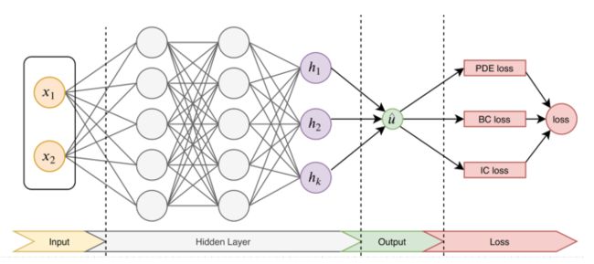
PINN的主要思想如图1,先构建一个输出结果为 u ^ \hat{u} u^的神经网络,将其作为PDE解的代理模型,将PDE信息作为约束,编码到神经网络损失函数中进行训练。损失函数主要包括4部分:偏微分结构损失(PDE loss),边值条件损失(BC loss)、初值条件损失(IC loss)以及真实数据条件损失(Data loss)。
特别的,考虑下面这个的PDE问题,其中PDE的解 u ( x ) u(x) u(x)在 Ω ⊂ R d \Omega \subset \mathbb{R}^{d} Ω⊂Rd定义,其中 x = ( x 1 , … , x d ) \mathbf{x}=\left(x_{1}, \ldots, x_{d}\right) x=(x1,…,xd):
f ( x ; ∂ u ∂ x 1 , … , ∂ u ∂ x d ; ∂ 2 u ∂ x 1 ∂ x 1 , … , ∂ 2 u ∂ x 1 ∂ x d ) = 0 , x ∈ Ω f\left(\mathbf{x} ; \frac{\partial u}{\partial x_{1}}, \ldots, \frac{\partial u}{\partial x_{d}} ; \frac{\partial^{2} u}{\partial x_{1} \partial x_{1}}, \ldots, \frac{\partial^{2} u}{\partial x_{1} \partial x_{d}} \right)=0, \quad \mathbf{x} \in \Omega f(x;∂x1∂u,…,∂xd∂u;∂x1∂x1∂2u,…,∂x1∂xd∂2u)=0,x∈Ω
同时,满足下面的边界
B ( u , x ) = 0 on ∂ Ω \mathcal{B}(u, \mathbf{x})=0 \quad \text { on } \quad \partial \Omega B(u,x)=0 on ∂Ω
PINN求解过程主要包括:
- 第一步,首先定义D层全连接层的神经网络模型:
N Θ : = L D ∘ σ ∘ L D − 1 ∘ σ ∘ ⋯ ∘ σ ∘ L 1 N_{\Theta}:=L_D \circ \sigma \circ L_{D-1} \circ \sigma \circ \cdots \circ \sigma \circ L_1 NΘ:=LD∘σ∘LD−1∘σ∘⋯∘σ∘L1
式中:
L 1 ( x ) : = W 1 x + b 1 , W 1 ∈ R d 1 × d , b 1 ∈ R d 1 L i ( x ) : = W i x + b i , W i ∈ R d i × d i − 1 , b i ∈ R d i , ∀ i = 2 , 3 , ⋯ D − 1 , L D ( x ) : = W D x + b D , W D ∈ R N × d D − 1 , b D ∈ R N . \begin{aligned} L_1(x) &:=W_1 x+b_1, \quad W_1 \in \mathbb{R}^{d_1 \times d}, b_1 \in \mathbb{R}^{d_1} \\ L_i(x) &:=W_i x+b_i, \quad W_i \in \mathbb{R}^{d_i \times d_{i-1}}, b_i \in \mathbb{R}^{d_i}, \forall i=2,3, \cdots D-1, \\ L_D(x) &:=W_D x+b_D, \quad W_D \in \mathbb{R}^{N \times d_{D-1}}, b_D \in \mathbb{R}^N . \end{aligned} L1(x)Li(x)LD(x):=W1x+b1,W1∈Rd1×d,b1∈Rd1:=Wix+bi,Wi∈Rdi×di−1,bi∈Rdi,∀i=2,3,⋯D−1,:=WDx+bD,WD∈RN×dD−1,bD∈RN.
以及 σ \sigma σ 为激活函数, W W W 和 b b b 为权重和偏差参数。 - 第二步,为了衡量神经网络 u ^ \hat{u} u^和约束之间的差异,考虑损失函数定义:
L ( θ ) = w f L P D E ( θ ; T f ) + w i L I C ( θ ; T i ) + w b L B C ( θ , ; T b ) + w d L D a t a ( θ , ; T d a t a ) \mathcal{L}\left(\boldsymbol{\theta}\right)=w_{f} \mathcal{L}_{PDE}\left(\boldsymbol{\theta}; \mathcal{T}_{f}\right)+w_{i} \mathcal{L}_{IC}\left(\boldsymbol{\theta} ; \mathcal{T}_{i}\right)+w_{b} \mathcal{L}_{BC}\left(\boldsymbol{\theta},; \mathcal{T}_{b}\right)+w_{d} \mathcal{L}_{Data}\left(\boldsymbol{\theta},; \mathcal{T}_{data}\right) L(θ)=wfLPDE(θ;Tf)+wiLIC(θ;Ti)+wbLBC(θ,;Tb)+wdLData(θ,;Tdata)
式中:
L P D E ( θ ; T f ) = 1 ∣ T f ∣ ∑ x ∈ T f ∥ f ( x ; ∂ u ^ ∂ x 1 , … , ∂ u ^ ∂ x d ; ∂ 2 u ^ ∂ x 1 ∂ x 1 , … , ∂ 2 u ^ ∂ x 1 ∂ x d ) ∥ 2 2 L I C ( θ ; T i ) = 1 ∣ T i ∣ ∑ x ∈ T i ∥ u ^ ( x ) − u ( x ) ∥ 2 2 L B C ( θ ; T b ) = 1 ∣ T b ∣ ∑ x ∈ T b ∥ B ( u ^ , x ) ∥ 2 2 L D a t a ( θ ; T d a t a ) = 1 ∣ T d a t a ∣ ∑ x ∈ T d a t a ∥ u ^ ( x ) − u ( x ) ∥ 2 2 \begin{aligned} \mathcal{L}_{PDE}\left(\boldsymbol{\theta} ; \mathcal{T}_{f}\right) &=\frac{1}{\left|\mathcal{T}_{f}\right|} \sum_{\mathbf{x} \in \mathcal{T}_{f}}\left\|f\left(\mathbf{x} ; \frac{\partial \hat{u}}{\partial x_{1}}, \ldots, \frac{\partial \hat{u}}{\partial x_{d}} ; \frac{\partial^{2} \hat{u}}{\partial x_{1} \partial x_{1}}, \ldots, \frac{\partial^{2} \hat{u}}{\partial x_{1} \partial x_{d}} \right)\right\|_{2}^{2} \\ \mathcal{L}_{IC}\left(\boldsymbol{\theta}; \mathcal{T}_{i}\right) &=\frac{1}{\left|\mathcal{T}_{i}\right|} \sum_{\mathbf{x} \in \mathcal{T}_{i}}\|\hat{u}(\mathbf{x})-u(\mathbf{x})\|_{2}^{2} \\ \mathcal{L}_{BC}\left(\boldsymbol{\theta}; \mathcal{T}_{b}\right) &=\frac{1}{\left|\mathcal{T}_{b}\right|} \sum_{\mathbf{x} \in \mathcal{T}_{b}}\|\mathcal{B}(\hat{u}, \mathbf{x})\|_{2}^{2}\\ \mathcal{L}_{Data}\left(\boldsymbol{\theta}; \mathcal{T}_{data}\right) &=\frac{1}{\left|\mathcal{T}_{data}\right|} \sum_{\mathbf{x} \in \mathcal{T}_{data}}\|\hat{u}(\mathbf{x})-u(\mathbf{x})\|_{2}^{2} \end{aligned} LPDE(θ;Tf)LIC(θ;Ti)LBC(θ;Tb)LData(θ;Tdata)=∣Tf∣1x∈Tf∑∥∥∥∥f(x;∂x1∂u^,…,∂xd∂u^;∂x1∂x1∂2u^,…,∂x1∂xd∂2u^)∥∥∥∥22=∣Ti∣1x∈Ti∑∥u^(x)−u(x)∥22=∣Tb∣1x∈Tb∑∥B(u^,x)∥22=∣Tdata∣1x∈Tdata∑∥u^(x)−u(x)∥22
w f w_{f} wf, w i w_{i} wi、 w b w_{b} wb和 w d w_{d} wd是权重。 T f \mathcal{T}_{f} Tf, T i \mathcal{T}_{i} Ti、 T b \mathcal{T}_{b} Tb和 T d a t a \mathcal{T}_{data} Tdata表示来自PDE,初值、边值以及真值的residual points。这里的 T f ⊂ Ω \mathcal{T}_{f} \subset \Omega Tf⊂Ω是一组预定义的点来衡量神经网络输出 u ^ \hat{u} u^与PDE的匹配程度。 - 最后,利用梯度优化算法最小化损失函数,直到找到满足预测精度的网络参数 KaTeX parse error: Undefined control sequence: \theat at position 1: \̲t̲h̲e̲a̲t̲^{*}。
值得注意的是,对于逆问题,即方程中的某些参数未知。若只知道PDE方程及边界条件,PDE参数未知,该逆问题为非定问题,所以必须要知道其他信息,如部分观测点 u u u 的值。在这种情况下,PINN做法可将方程中的参数作为未知变量,加到训练器中进行优化,损失函数包括Data loss。
3.求解问题定义—正问题
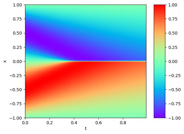
u t + u u x = v u x x , x ∈ [ − 1 , 1 ] , t > 0 u ( x , 0 ) = − sin ( π x ) u ( − 1 , t ) = u ( 1 , t ) = 0 \begin{aligned} u_t+u u_x &=v u_{x x}, x \in[-1,1], t>0 \\ u(x, 0) &=-\sin (\pi x) \\ u(-1, t) &=u(1, t)=0 \end{aligned} ut+uuxu(x,0)u(−1,t)=vuxx,x∈[−1,1],t>0=−sin(πx)=u(1,t)=0
式中:参数 v ∈ [ 0 , 0.1 / π ] v \in[0,0.1 / \pi] v∈[0,0.1/π]。数值解通过Hopf-Cole transformation获得,如图2。
任务要求:
- 该任务为已知边界条件和微分方程求解u。
4.Python求解代码
Burger方程仿真数据下载地址
- 第一步,首先定义神经网络。这里和之前网络不同点主要在于,网络中增加了可训练参数 a。
import torch
import torch.optim
from collections import OrderedDict
import torch.nn as nn

class Net(nn.Module):
    def __init__(self, seq_net, name='MLP', activation=torch.tanh):
        super().__init__()
        self.features = OrderedDict()
        for i in range(len(seq_net) - 1):
            self.features['{}_{}'.format(name, i)] = nn.Linear(seq_net[i], seq_net[i + 1], bias=True)
        self.features = nn.ModuleDict(self.features)
        self.active = activation

        # initial_bias
        for m in self.modules():
            if isinstance(m, nn.Linear):
                nn.init.constant_(m.bias, 0)

    def forward(self, x):
        # x = x.view(-1, 2)
        length = len(self.features)
        i = 0
        for name, layer in self.features.items():
            x = layer(x)
            if i == length - 1: break
            i += 1
            x = self.active(x)
        return x
- 第二步,PINN求解框架,定义网络,采点构建损失函数,优化器优化损失函数。这里和深度学习求解微分方程系列二:PINN求解burger方程,不同点主要在于多了Data loss项,同时PDE未知参数被加入网络优化器中进行训练。
from net import Net
import torch
from torch.autograd import grad
import os
import matplotlib.pyplot as plt
import scipy.io
import numpy as np
from math import pi
def d(f, x):
return grad(f, x, grad_outputs=torch.ones_like(f), create_graph=True, only_inputs=True)[0]
def PDE(u, t, x, nu):
return d(u, t) + u * d(u, x) - nu * d(d(u, x), x)
def train():
# Parameter setting
nu = 0.01 / pi
lr = 0.001
epochs = 12000
t_left, t_right = 0., 1.
x_left, x_right = -1., 1.
n_f, n_b_1, n_b_2 = 10000, 5000, 5000
# test data
data = scipy.io.loadmat('./result/burgers_shock.mat')
Exact = np.real(data['usol']).T
t = data['t'].flatten()[:, None]
x = data['x'].flatten()[:, None]
X, T = np.meshgrid(x, t)
s_shape = X.shape
X_star = np.hstack((X.flatten()[:, None], T.flatten()[:, None])) # 在水平方向上平铺(25600, 2)
X_star = X_star.astype(np.float32)
X_star = torch.from_numpy(X_star).cuda().requires_grad_(True)
u_star = Exact.flatten()[:, None]
u_star = u_star.astype(np.float32)
u_star = torch.from_numpy(u_star).cuda().requires_grad_(True)
os.environ['CUDA_VISIBLE_DEVICES'] = '0'
device = torch.device('cuda:0') if torch.cuda.is_available() else torch.cuda('cpu')
PINN = Net(seq_net=[2, 20, 20, 20, 20, 20, 20, 1], activation=torch.tanh).to(device)
optimizer = torch.optim.Adam(PINN.parameters(), lr)
criterion = torch.nn.MSELoss()
loss_history = []
mse_loss = []
for epoch in range(epochs):
optimizer.zero_grad()
# inside
t_f = ((t_left + t_right) / 2 + (t_right - t_left) *
(torch.rand(size=(n_f, 1), dtype=torch.float, device=device) - 0.5)
).requires_grad_(True)
x_f = ((x_left + x_right) / 2 + (x_right - x_left) *
(torch.rand(size=(n_f, 1), dtype=torch.float, device=device) - 0.5)
).requires_grad_(True)
u_f = PINN(torch.cat([t_f, x_f], dim=1))
PDE_ = PDE(u_f, t_f, x_f, nu)
mse_PDE = criterion(PDE_, torch.zeros_like(PDE_))
# boundary
x_rand = ((x_left + x_right) / 2 + (x_right - x_left) *
(torch.rand(size=(n_b_1, 1), dtype=torch.float, device=device) - 0.5)
).requires_grad_(True)
t_b = (t_left * torch.ones_like(x_rand)
).requires_grad_(True)
u_b_1 = PINN(torch.cat([t_b, x_rand], dim=1)) + torch.sin(pi * x_rand)
t_rand = ((t_left + t_right) / 2 + (t_right - t_left) *
(torch.rand(size=(n_b_2, 1), dtype=torch.float, device=device) - 0.5)
).requires_grad_(True)
x_b_1 = (x_left * torch.ones_like(t_rand)
).requires_grad_(True)
x_b_2 = (x_right * torch.ones_like(t_rand)
).requires_grad_(True)
u_b_2 = PINN(torch.cat([t_rand, x_b_1], dim=1))
u_b_3 = PINN(torch.cat([t_rand, x_b_2], dim=1))
mse_BC_1 = criterion(u_b_1, torch.zeros_like(u_b_1))
mse_BC_2 = criterion(u_b_2, torch.zeros_like(u_b_2))
mse_BC_3 = criterion(u_b_3, torch.zeros_like(u_b_3))
mse_BC = mse_BC_1 + mse_BC_2 + mse_BC_3
# loss
loss = 1 * mse_PDE + 1 * mse_BC
# Pred loss
x_pred = X_star[:, 0:1]
t_pred = X_star[:, 1:2]
u_pred = PINN(torch.cat([t_pred, x_pred], dim=1))
mse_test = criterion(u_pred, u_star)
loss_history.append([mse_PDE.item(), mse_BC.item(), mse_test.item()])
mse_loss.append(loss.item())
if (epoch + 1) % 1000 == 0:
print(
'epoch:{:05d}, PDE: {:.08e}, BC: {:.08e}, loss: {:.08e}'.format(
epoch, mse_PDE.item(), mse_BC.item(), loss.item()
)
)
loss.backward()
optimizer.step()
# Plotting
if (epoch + 1) % 2000 == 0:
plt.cla()
fig = plt.figure(figsize=(12, 4))
xx = torch.linspace(0, 1, 1000).cpu()
yy = torch.linspace(-1, 1, 1000).cpu()
x1, y1 = torch.meshgrid([xx, yy])
s1 = x1.shape
x1 = x1.reshape((-1, 1))
y1 = y1.reshape((-1, 1))
out = torch.cat([x1, y1], dim=1).to(device)
z = PINN(out)
z_out = z.reshape(s1)
out = z_out.cpu().T.detach().numpy()
plt.pcolormesh(xx, yy, out, cmap='rainbow')
cbar = plt.colorbar(pad=0.05, aspect=10)
cbar.mappable.set_clim(-1, 1)
plt.xticks([])
plt.yticks([])
# plt.savefig('./result_plot/Burger1d_pred_{}.png'.format(epoch + 1), bbox_inches='tight', format='png')
plt.show()
x_pred = X_star[:, 0:1]
t_pred = X_star[:, 1:2]
u_pred = PINN(torch.cat([t_pred, x_pred], dim=1))
plt.pcolormesh(np.squeeze(t, axis=1), np.squeeze(x, axis=1),
u_pred.cpu().detach().numpy().reshape(s_shape).T, cmap='rainbow')
cbar = plt.colorbar(pad=0.05, aspect=10)
cbar.mappable.set_clim(-1, 1)
plt.xticks([])
plt.yticks([])
plt.savefig('./result_plot/Burger1d_pred_{}.png'.format(epoch + 1), bbox_inches='tight', format='png')
plt.show()
plt.cla()
mse_test = abs(u_pred - u_star)
plt.pcolormesh(np.squeeze(t, axis=1), np.squeeze(x, axis=1),
mse_test.cpu().detach().numpy().reshape(s_shape).T, cmap='rainbow')
cbar = plt.colorbar(pad=0.05, aspect=10)
cbar.mappable.set_clim(0, 0.3)
plt.xticks([])
plt.yticks([])
plt.savefig('./result_plot/Burger1d_error_{}.png'.format(epoch + 1), bbox_inches='tight', format='png')
plt.show()
#
fig, ax = plt.subplots(1, 3, figsize=(12, 4))
x_25 = x.astype(np.float32)
x_25 = torch.from_numpy(x_25).cuda().requires_grad_(True)
t_25 = (0.25 * torch.ones_like(x_25)).requires_grad_(True)
u_25 = PINN(torch.cat([t_25, x_25], dim=1))
ax[0].plot(x, Exact[25, :], 'b-', linewidth=2)
ax[0].plot(x, u_25.reshape((-1, 1)).detach().cpu().numpy(), 'r-', linewidth=2, linestyle='-',
label='PINN', )
ax[0].set_xlabel('x')
ax[0].set_ylabel('u(t,x)')
ax[0].axis('square')
ax[0].set_xlim([-1.1, 1.1])
ax[0].set_ylim([-1.1, 1.1])
ax[0].set_title('t = 0.25', fontsize=10)
t_50 = (0.5 * torch.ones_like(x_25)).requires_grad_(True)
u_50 = PINN(torch.cat([t_50, x_25], dim=1))
ax[1].plot(x, Exact[50, :], 'b-', linewidth=2, label='Exact')
ax[1].plot(x, u_50.reshape((-1, 1)).detach().cpu().numpy(), 'r-', linewidth=2, label='PINN',
linestyle='--')
ax[1].set_xlabel('x')
ax[1].set_ylabel('u(t,x)')
ax[1].axis('square')
ax[1].set_xlim([-1.1, 1.1])
ax[1].set_ylim([-1.1, 1.1])
ax[1].set_title('t = 0.50', fontsize=10)
ax[1].legend(loc='upper center', bbox_to_anchor=(0.5, -0.1), ncol=5, frameon=False)
t_75 = (0.75 * torch.ones_like(x_25)).requires_grad_(True)
u_75 = PINN(torch.cat([t_75, x_25], dim=1))
ax[2].plot(x, Exact[75, :], 'b-', linewidth=2)
ax[2].plot(x, u_75.reshape((-1, 1)).detach().cpu().numpy(), 'r-', linestyle='--', linewidth=2, label='PINN')
ax[2].set_xlabel('x')
ax[2].set_ylabel('u(t,x)')
ax[2].axis('square')
ax[2].set_xlim([-1.1, 1.1])
ax[2].set_ylim([-1.1, 1.1])
ax[2].set_title('t = 0.75', fontsize=10)
plt.savefig('./result_plot/Burger1d_t_{}.png'.format(epoch + 1), bbox_inches='tight', format='png')
plt.show()
plt.cla()
plt.plot(loss_history)
plt.yscale('log')
plt.ylim(1e-5, 1)
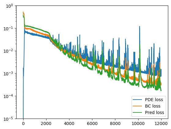
plt.legend(('PDE loss', 'BC loss', 'Pred loss'), loc='best')
plt.savefig('./result_plot/Burger1d_loss_{}.png'.format(epochs + 1), bbox_inches='tight', format='png')
plt.show()
if __name__ == '__main__':
train()
5.结果展示
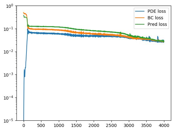
预测结果如图3-5所示。此外值得注意的是该算法对网络采用随机初始化,当初始化不好时,就会出现图5所示的训练误差。
训练过程中预测结果图如图4-5。