吴恩达机器学习ex3 python实现

多分类

这个部分需要你实现手写数字（0到9）的识别。你需要扩展之前的逻辑回归，并将其应用于一对多的分类。

数据集

这是一个MATLAB格式的.m文件，其中包含5000个20*20像素的手写字体图像，以及他对应的数字。另外，数字0的y值，对应的是10
用Python读取我们需要使用SciPy

import numpy as np
import pandas as pd
import matplotlib.pyplot as plt
import matplotlib
from scipy.io import loadmat
from sklearn.metrics import classification_report

data = loadmat('ex3data1.mat')
data

{'X': array([[0., 0., 0., ..., 0., 0., 0.],
        [0., 0., 0., ..., 0., 0., 0.],
        [0., 0., 0., ..., 0., 0., 0.],
        ...,
        [0., 0., 0., ..., 0., 0., 0.],
        [0., 0., 0., ..., 0., 0., 0.],
        [0., 0., 0., ..., 0., 0., 0.]]),
 '__globals__': [],
 '__header__': b'MATLAB 5.0 MAT-file, Platform: GLNXA64, Created on: Sun Oct 16 13:09:09 2011',
 '__version__': '1.0',
 'y': array([[10],
        [10],
        [10],
        ...,
        [ 9],
        [ 9],
        [ 9]], dtype=uint8)}

data['X'].shape ,data['y'].shape

((5000, 400), (5000, 1))

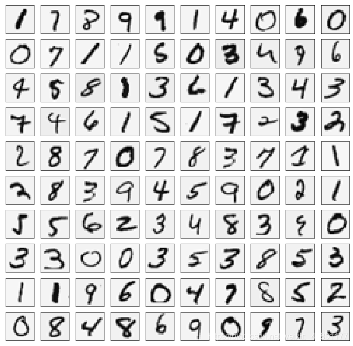
数据可视化

随机展示100个数据

sample_idx = np.random.choice(np.arange(data['X'].shape[0]),100)
sample_images = data['X'][sample_idx,:]
sample_images

array([[0., 0., 0., ..., 0., 0., 0.],
       [0., 0., 0., ..., 0., 0., 0.],
       [0., 0., 0., ..., 0., 0., 0.],
       ...,
       [0., 0., 0., ..., 0., 0., 0.],
       [0., 0., 0., ..., 0., 0., 0.],
       [0., 0., 0., ..., 0., 0., 0.]])

fig,ax_array = plt.subplots(nrows=10,ncols=10,sharey=True,sharex=True,figsize=(12,12))
for r in range(10):
    for c in range(10):
        ax_array[r,c].matshow(np.array(sample_images[10*r+c].reshape((20,20))).T,cmap=matplotlib.cm.binary)
        plt.xticks(np.array([]))
        plt.yticks(np.array([]))

将逻辑回归向量化

你将用多分类逻辑回归做一个分类器。因为现在有10个数字类别，所以你需要训练10个不同的逻辑回归分类器。为了让训练效率更高，将逻辑回归向量化是非常重要的，不要用循环。

向量化代价函数J($\theta$)

def sigmoid(z):
    return 1/(1+np.exp(-z))

#向量化代价函数
def cost(theta,X,y,learningRate):
    theta = np.matrix(theta)
    X = np.matrix(X)
    y = np.matrix(y)
    
    left = np.multiply(-y,np.log(sigmoid(X*theta.T)))
    right = np.multiply((1-y),np.log(1-sigmoid(X*theta.T)))
    reg = (learningRate/(2*len(X)))*np.sum(np.power(theta[:,1:theta.shape[1]],2))
    return np.sum(left-right)/len(X) + reg

向量化正则化逻辑回归

#向量化梯度函数
def gradient(theta,X,y,learningRate):
    theta = np.matrix(theta)
    X = np.matrix(X)
    y = np.matrix(y)
    
    parameters = int(theta.ravel().shape[1])
    error = sigmoid(X*theta.T) - y
    
    grad = ((X.T * error)/len(X)).T + ((learningRate/len(X))*theta) 
    
    grad[0,0] = np.sum(np.multiply(error,X[:,0]))/len(X)
    
    return np.array(grad).ravel()

一对多分类器

现在我们已经定义了代价函数和梯度函数，现在是构建分类器的时候了。
对于这个任务，我们有10个可能的类，并且由于逻辑回归只能一次在2个类之间进行分类，我们需要多类分类的策略。
在本练习中，我们的任务是实现一对一全分类方法，其中具有k个不同类的标签就有k个分类器，每个分类器在“类别 i”和“不是 i”之间决定。
我们将把分类器训练包含在一个函数中，该函数计算10个分类器中的每个分类器的最终权重，并将权重返回为k*(n + 1)数组，其中n是参数数量。

from scipy.optimize import minimize
#单层网络模型
def one_vs_all(X,y,num_labels,learning_rate):
    rows = X.shape[0]
    params = X.shape[1]
    
    #k*(n+1) 的array，用于储存每个k分类器的参数
    all_theta = np.zeros((num_labels,params+1))
    
    #插入一列1
    X = np.insert(X,0,values=np.ones(rows),axis=1)
    
    #labels都是以1开始索引的，不是从0
    for i in range(1,num_labels+1):
        theta = np.zeros(params+1)
        #相当于新建一个二分类器的数据，输入不变，输出变为是否为i的二分类
        y_i = np.array([1 if label == i else 0 for label in y])
        y_i = np.reshape(y_i,(rows,1))
        
        #最优化代价函数
        fmin = minimize(fun = cost, x0 = theta,args = (X,y_i,learning_rate),method = 'TNC',jac = gradient)
        all_theta[i-1,:] = fmin.x
        
    return all_theta

这里需要注意的几点：首先，我们为theta添加了一个额外的参数（与训练数据一列），以计算截距项（常数项）。 其次，我们将y从类标签转换为每个分类器的二进制值（要么是类i，要么不是类i）。 最后，我们使用SciPy的较新优化API来最小化每个分类器的代价函数。 如果指定的话，API将采用目标函数，初始参数集，优化方法和jacobian（渐变）函数。 然后将优化程序找到的参数分配给参数数组。

实现向量化代码的一个更具挑战性的部分是正确地写入所有的矩阵，保证维度正确。

rows = data['X'].shape[0]
params = data['X'].shape[1]

all_theta = np.zeros((10,params + 1))

X = np.insert(data['X'],0,values=np.ones(rows),axis=1)

theta = np.zeros(params+1)

y_0 = np.array([1 if label == 0 else 0 for label in data['y']])
y_0 = np.reshape(y_0,(rows,1))

X.shape,y_0.shape,theta.shape,all_theta.shape

((5000, 401), (5000, 1), (401,), (10, 401))

注意，theta是一维数组，因此当它被转换为计算梯度的代码中的矩阵时，它变为（1×401）矩阵。 我们还检查y中的类标签，以确保它们看起来像我们想象的一致。

#查看y中有几类
np.unique(data['y'])

array([ 1,  2,  3,  4,  5,  6,  7,  8,  9, 10], dtype=uint8)

all_theta = one_vs_all(data['X'],data['y'],10,1)
all_theta

array([[-2.38254176e+00,  0.00000000e+00,  0.00000000e+00, ...,
         1.30426303e-03, -7.17245139e-10,  0.00000000e+00],
       [-3.18255097e+00,  0.00000000e+00,  0.00000000e+00, ...,
         4.46037881e-03, -5.08528248e-04,  0.00000000e+00],
       [-4.79725016e+00,  0.00000000e+00,  0.00000000e+00, ...,
        -2.87026543e-05, -2.47433759e-07,  0.00000000e+00],
       ...,
       [-7.98553657e+00,  0.00000000e+00,  0.00000000e+00, ...,
        -8.95420362e-05,  7.21788914e-06,  0.00000000e+00],
       [-4.57378972e+00,  0.00000000e+00,  0.00000000e+00, ...,
        -1.33558726e-03,  9.98591236e-05,  0.00000000e+00],
       [-5.40484816e+00,  0.00000000e+00,  0.00000000e+00, ...,
        -1.16513518e-04,  7.86318240e-06,  0.00000000e+00]])

一对多预测

我们现在准备好最后一步 - 使用训练完毕的分类器预测每个图像的标签。 对于这一步，我们将计算每个类的类概率，对于每个训练样本（使用当然的向量化代码），并将输出类标签为具有最高概率的类。

def predict_all(X,all_theta):
    rows = X.shape[0]
    params = X.shape[1]
    num_labels = all_theta.shape[0]
    
    #插入常数项1
    X = np.insert(X,0,values=np.ones(rows),axis=1)
    X = np.matrix(X)
    all_theta = np.matrix(all_theta)
    
    #计算每个样本的分类可能性
    h = sigmoid(X*all_theta.T)
    
    #创建每个样本最大可能是的数字的array
    h_argmax = np.argmax(h,axis = 1)
    h_argmax = h_argmax + 1 #因为我们是以0开始的
    
    return h_argmax

现在我们可以使用predict_all函数为每个实例生成类预测，看看我们的分类器是如何工作的。

y_pred = predict_all(data['X'],all_theta)
print(classification_report(data['y'],y_pred))

              precision    recall  f1-score   support

           1       0.95      0.99      0.97       500
           2       0.95      0.92      0.93       500
           3       0.95      0.91      0.93       500
           4       0.95      0.95      0.95       500
           5       0.92      0.92      0.92       500
           6       0.97      0.98      0.97       500
           7       0.95      0.95      0.95       500
           8       0.93      0.92      0.92       500
           9       0.92      0.92      0.92       500
          10       0.97      0.99      0.98       500

    accuracy                           0.94      5000
   macro avg       0.94      0.94      0.94      5000
weighted avg       0.94      0.94      0.94      5000

神经网络

在前面一个部分，我们已经实现了多分类逻辑回归来识别手写数字。但是，逻辑回归并不能承载更复杂的假设，因为他就是个线性分类器。
这部分，你需要实现一个可以识别手写数字的神经网络。神经网络可以表示一些非线性复杂的模型。权重已经预先训练好，你的目标是在现有权重基础上，实现前馈神经网络。

模型表达

输入是图片的像素值，20*20像素的图片有400个输入层单元，不包括需要额外添加的加上常数项。
材料已经提供了训练好的神经网络的参数${\Theta }^{(1)}$,${\Theta }^{(2)}$，有25个隐层单元和10个输出单元（10个输出）

前馈神经网络和预测

你需要实现前馈神经网络预测手写数字的功能。和之前的一对多分类一样，神经网络的预测会把$(h_{\theta }(x){)}_k$中值最大的，作为预测输出

weight = loadmat("ex3weights.mat")
theta1,theta2 = weight['Theta1'],weight['Theta2']
theta1.shape,theta2.shape

((25, 401), (10, 26))

#插入常数项
X2 = np.matrix(np.insert(data['X'],0,values=np.ones(X.shape[0]),axis=1))
y2 = np.matrix(data['y'])
X2.shape,y2.shape

((5000, 401), (5000, 1))

a1 = X2
z2 = a1*theta1.T
z2.shape

(5000, 25)

a2 = sigmoid(z2)
a2.shape

(5000, 25)

a2 = np.insert(a2,0,np.ones(a2.shape[0]),axis = 1)
z3 = a2*theta2.T
z3.shape

(5000, 10)

a3 = sigmoid(z3)
a3

matrix([[1.12661530e-04, 1.74127856e-03, 2.52696959e-03, ...,
         4.01468105e-04, 6.48072305e-03, 9.95734012e-01],
        [4.79026796e-04, 2.41495958e-03, 3.44755685e-03, ...,
         2.39107046e-03, 1.97025086e-03, 9.95696931e-01],
        [8.85702310e-05, 3.24266731e-03, 2.55419797e-02, ...,
         6.22892325e-02, 5.49803551e-03, 9.28008397e-01],
        ...,
        [5.17641791e-02, 3.81715020e-03, 2.96297510e-02, ...,
         2.15667361e-03, 6.49826950e-01, 2.42384687e-05],
        [8.30631310e-04, 6.22003774e-04, 3.14518512e-04, ...,
         1.19366192e-02, 9.71410499e-01, 2.06173648e-04],
        [4.81465717e-05, 4.58821829e-04, 2.15146201e-05, ...,
         5.73434571e-03, 6.96288990e-01, 8.18576980e-02]])

y_pred2 = np.argmax(a3,axis=1) + 1
y_pred2.shape

(5000, 1)

print(classification_report(y2,y_pred2))

              precision    recall  f1-score   support

           1       0.97      0.98      0.98       500
           2       0.98      0.97      0.98       500
           3       0.98      0.96      0.97       500
           4       0.97      0.97      0.97       500
           5       0.97      0.98      0.98       500
           6       0.98      0.99      0.98       500
           7       0.98      0.97      0.97       500
           8       0.98      0.98      0.98       500
           9       0.97      0.96      0.96       500
          10       0.98      0.99      0.99       500

    accuracy                           0.98      5000
   macro avg       0.98      0.98      0.98      5000
weighted avg       0.98      0.98      0.98      5000