马尔可夫决策过程

Markov decision process

From Wikipedia, the free encyclopedia

Markov decision processes (MDPs), named after Andrey Markov, provide a mathematical framework for modeling decision making in situations where outcomes are partly random and partly under the control of a decision maker. MDPs are useful for studying a wide range of optimization problems solved via dynamic programming and reinforcement learning. MDPs were known at least as early as the 1950s (cf. Bellman 1957). A core body of research on Markov decision processes resulted from Ronald A. Howard's book published in 1960, Dynamic Programming and Markov Processes. They are used in a wide area of disciplines, including robotics, automated control, economics, and manufacturing.

More precisely, a Markov Decision Process is a discrete time stochastic control process. At each time step, the process is in some state , and the decision maker may choose any action  that is available in state . The process responds at the next time step by randomly moving into a new state , and giving the decision maker a corresponding reward .

The probability that the process moves into its new state  is influenced by the chosen action. Specifically, it is given by the state transition function . Thus, the next state  depends on the current state  and the decision maker's action . But given  and , it is conditionally independent of all previous states and actions; in other words, the state transitions of an MDP possess the Markov property.

Markov decision processes are an extension of Markov chains; the difference is the addition of actions (allowing choice) and rewards (giving motivation). Conversely, if only one action exists for each state and all rewards are zero, a Markov decision process reduces to a Markov chain.

[edit]Definition

Example of a simple MDP with three states and two actions.

A Markov decision process is a 4-tuple , where

•  is a finite set of states,
•  is a finite set of actions (alternatively,  is the finite set of actions available from state ),
•  is the probability that action  in state  at time  will lead to state  at time ,
•  is the immediate reward (or expected immediate reward) received after transition to state  from state  with transition probability .

(The theory of Markov decision processes does not actually require  or to be finite,^{[citation needed]} but the basic algorithms below assume that they are finite.)

[edit]Problem

The core problem of MDPs is to find a "policy" for the decision maker: a function  that specifies the action  that the decision maker will choose when in state . Note that once a Markov decision process is combined with a policy in this way, this fixes the action for each state and the resulting combination behaves like a Markov chain.

The goal is to choose a policy  that will maximize some cumulative function of the random rewards, typically the expected discounted sum over a potentially infinite horizon:

    (where we choose  )

where  is the discount factor and satisfies . (For example,  when the discount rate is r.)  is typically close to 1.

Because of the Markov property, the optimal policy for this particular problem can indeed be written as a function of  only, as assumed above.

[edit]Algorithms

MDPs can be solved by linear programming or dynamic programming. In what follows we present the latter approach.

Suppose we know the state transition function  and the reward function , and we wish to calculate the policy that maximizes the expected discounted reward.

The standard family of algorithms to calculate this optimal policy requires storage for two arrays indexed by state: value , which contains real values, and policy  which contains actions. At the end of the algorithm,  will contain the solution and  will contain the discounted sum of the rewards to be earned (on average) by following that solution from state .

The algorithm has the following two kinds of steps, which are repeated in some order for all the states until no further changes take place. They are

Their order depends on the variant of the algorithm; one can also do them for all states at once or state by state, and more often to some states than others. As long as no state is permanently excluded from either of the steps, the algorithm will eventually arrive at the correct solution.

[edit]Notable variants

[edit]Value iteration

In value iteration (Bellman 1957), which is also called backward induction, the  array is not used; instead, the value of  is calculated whenever it is needed. Shapley's 1953 paper on stochastic games included as a special case the value iteration method for MDPs, but this was recognized only later on.^[1]

Substituting the calculation of  into the calculation of  gives the combined step:

This update rule is iterated for all states  until it converges with the left-hand side equal to the right-hand side (which is the "Bellman equation" for this problem).

[edit]Policy iteration

In policy iteration (Howard 1960), step one is performed once, and then step two is repeated until it converges. Then step one is again performed once and so on.

Instead of repeating step two to convergence, it may be formulated and solved as a set of linear equations.

This variant has the advantage that there is a definite stopping condition: when the array  does not change in the course of applying step 1 to all states, the algorithm is completed.

[edit]Modified policy iteration

In modified policy iteration (van Nunen, 1976; Puterman and Shin 1978), step one is performed once, and then step two is repeated several times. Then step one is again performed once and so on.

[edit]Prioritized sweeping

In this variant, the steps are preferentially applied to states which are in some way important - whether based on the algorithm (there were large changes in  or  around those states recently) or based on use (those states are near the starting state, or otherwise of interest to the person or program using the algorithm).

[edit]Extensions and generalizations

A Markov decision process is a stochastic game with only one player.

[edit]Partial observability

Main article:  partially observable Markov decision process

The solution above assumes that the state  is known when action is to be taken; otherwise  cannot be calculated. When this assumption is not true, the problem is called a partially observable Markov decision process or POMDP.

A major breakthrough in this area was provided in "Optimal adaptive policies for Markov decision processes" ^[2] by Burnetas and Katehakis. In this work a class of adaptive policies that possess uniformly maximum convergence rate properties for the total expected finite horizon reward, were constructed under the assumptions of finite state-action spaces and irreducibility of the transition law. These policies prescribe that the choice of actions, at each state and time period, should be based on indices that are inflations of the right-hand side of the estimated average reward optimality equations.

[edit]Reinforcement learning

If the probabilities or rewards are unknown, the problem is one of reinforcement learning (Sutton and Barto, 1998).

For this purpose it is useful to define a further function, which corresponds to taking the action  and then continuing optimally (or according to whatever policy one currently has):

While this function is also unknown, experience during learning is based on  pairs (together with the outcome ); that is, "I was in state  and I tried doing  and  happened"). Thus, one has an array  and uses experience to update it directly. This is known asQ‑learning.

Reinforcement learning can solve Markov decision processes without explicit specification of the transition probabilities; the values of the transition probabilities are needed in value and policy iteration. In reinforcement learning, instead of explicit specification of the transition probabilities, the transition probabilities are accessed through a simulator that is typically restarted many times from a uniformly random initial state. Reinforcement learning can also be combined with function approximation to address problems with a very large number of states.

[edit]Continuous-time Markov Decision Process

In discrete-time Markov Decision Processes, decisions are made at discrete time epoch. However, for Continuous-time Markov Decision Process, decisions can be made at any time when decision maker wants. Unlike discrete-time Markov Decision Process, Continuous-time Markov Decision Process could better model the decision making process when the interested system has continuous dynamics, i.e., the system dynamics is defined by partial differential equations (PDEs).

[edit]Definition

In order to discuss the continuous-time Markov Decision Process, we introduce two sets of notations:

If the state space and action space are finite,

• : State space;
• : Action space;
• : , transition rate function;
• : , a reward function.

If the state space and action space are continuous,

• : State space.;
• : Space of possible control;
• : , a transition rate function;
• : , a reward rate function such that , where  is the reward function we discussed in previous case.

[edit]Problem

Like the Discrete-time Markov Decision Processes, in Continuous-time Markov Decision Process we want to find the optimal policy or controlwhich could give us the optimal expected integrated reward:

Where 

[edit]Linear programming formulation

If the state space and action space are finite, we could use linear programming formulation to find the optimal policy, which was one of the earliest solution approaches. Here we only consider the ergodic model, which means our continuous-time MDP becomes an ergodic continuous-time Markov Chain under a stationary policy. Under this assumption, although the decision maker could make decision at any time, on the current state, he could not get more benefit to make more than one actions. It is better for him to take action only at the time when system transit from current state to another state. Under some conditions,(for detail check Corollary 3.14 of Continuous-Time Markov Decision Processes), if our optimal value function  is independent of state i, we will have a following equation:

If there exists a function , then  will be the smallest g could satisfied the above equation. In order to find the , we could have the following linear programming model:

• Primal linear program(P-LP)

• Dual linear program(D-LP)

 is a feasible solution to the D-LP if  is nonnative and satisfied the constraints in the D-LP problem. A feasible solution  to the D-LP is said to be an optimal solution if

for all feasible solution y(i,a) to the D-LP. Once we found the optimal solution , we could use those optimal solution to establish the optimal policies.

[edit]Hamilton-Jacobi-Bellman equation

In continuous-time MDP, if the state space and action space are continuous, the optimal criterion could be found by solving Hamilton-Jacobi-Bellman (HJB) partial differential equation. In order to discuss the HJB equation, we need to reformulate our problem

D() is the terminal reward function,  is the system state vector,  is the system control vector we try to find. f() shows how the state vector change over time. Hamilton-Jacobi-Bellman equation is as follows:

We could solve the equation to find the optimal control , which could give us the optimal value 

[edit]Application

Queueing system, epidemic processes, Population process.

[edit]Alternative notations

The terminology and notation for MDPs are not entirely settled. There are two main streams — one focuses on maximization problems from contexts like economics, using the terms action, reward, value, and calling the discount factor  or , while the other focuses on minimization problems from engineering and navigation, using the terms control, cost, cost-to-go, and calling the discount factor . In addition, the notation for the transition probability varies.

in this article	alternative	comment
action	control
reward	cost	is the negative of
value	cost-to-go	is the negative of
policy	policy
discounting factor	discounting factor
transition probability	transition probability

In addition, transition probability is sometimes written ,  or, rarely, 

[edit]See also

• Partially observable Markov decision process
• Dynamic programming
• Bellman equation for applications to economics.
• Hamilton–Jacobi–Bellman equation
• Optimal control

[edit]Notes

1. ^ Lodewijk Kallenberg, Finite state and action MDPs, in Eugene A. Feinberg, Adam Shwartz (eds.) Handbook of Markov decision processes: methods and applications, Springer, 2002, ISBN 0-7923-7459-2
2. ^ Burnetas AN and Katehakis MN (1997). "Optimal adaptive policies for Markov decision processes", Math. Oper. Res., 22(1), 262–268

[edit]References

• R. Bellman. A Markovian Decision Process. Journal of Mathematics and Mechanics 6, 1957.
• R. E. Bellman. Dynamic Programming. Princeton University Press, Princeton, NJ, 1957. Dover paperback edition (2003), ISBN 0-486-42809-5.
• Ronald A. Howard Dynamic Programming and Markov Processes, The M.I.T. Press, 1960.
• D. Bertsekas. Dynamic Programming and Optimal Control. Volume 2, Athena, MA, 1995.
• Burnetas, A.N. and M. N. Katehakis. "Optimal Adaptive Policies for Markov Decision Processes, Mathematics of Operations Research, 22,(1), 1995.
• M. L. Puterman. Markov Decision Processes. Wiley, 1994.
• H.C. Tijms. A First Course in Stochastic Models. Wiley, 2003.
• Sutton, R. S. and Barto A. G. Reinforcement Learning: An Introduction. The MIT Press, Cambridge, MA, 1998.
• J.A. E. E van Nunen. A set of successive approximation methods for discounted Markovian decision problems. Z. Operations Research, 20:203-208, 1976.
• S. P. Meyn, 2007. Control Techniques for Complex Networks, Cambridge University Press, 2007. ISBN 978-0-521-88441-9. Appendix contains abridged Meyn & Tweedie.
• S. M. Ross. 1983. Introduction to stochastic dynamic programming. Academic press
• X. Guo and O. Hernández-Lerma. Continuous-Time Markov Decision Processes, Springer, 2009.
• M. L. Puterman and Shin M. C. Modified Policy Iteration Algorithms for Discounted Markov Decision Problems, Management Science 24, 1978.

马尔可夫决策过程（MDPs）以安德烈马尔可夫的名字命名 ，针对一些决策的输出结果部分随机而又部分可控的情况，给决策者提供一个决策制定的数学建模框架。MDPs对通过动态规划和强化学习来求解的广泛的优化问题是非常有用的。MDPs至少早在20世纪50年代就被大家熟知（参见贝尔曼1957年）。大部分MDPs领域的研究产生于罗纳德.A.霍华德1960年出版的《动态规划与马尔可夫过程》。今天，它们被应用在各种领域，包括机器人技术，自动化控制，经济和制造业领域。

更确切地说，一个马尔可夫决策过程是一个离散时间随机控制的过程。在每一个时阶（each time step），此决策过程处于某种状态 s ，决策者可以选择在状态 s 下可用的任何动作 a。该过程在下一个时阶做出反应随机移动到一个新的状态 s'，并给予决策者相应的奖励 Ra(s,s')。

此过程选择 s'作为其新状态的概率又受到所选择动作的影响。具体来说，此概率由状态转变函数Pa(s,s')来规定。因此，下一个状态 s' 取决于当前状态 s 和决策者的动作 a 。但是考虑到状态 s和动作 a，不依赖以往所有的状态和动作是有条件的，换句话说，一个的MDP状态转换具有马尔可夫特性。

马尔可夫决策过程是一个马尔可夫链的扩展；区别是动作（允许选择）和奖励（给予激励）的加入。相反，如果忽视奖励，即使每一状态只有一个动作存在，那么马尔可夫决策过程即简化为一个马尔可夫链。

定义

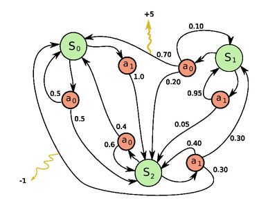
一个很简单的只有3个状态和2个动作的MDP例子。

 

一个马尔可夫决策过程是一个4 - 元组 ，其中

                      S是状态的有限集合，

                      A是动作的有限集合（或者，As是处于状态s下可用的一组动作的有限集合），

                     表示 t时刻的动作 a 将导致马尔可夫过程由状态 s 在t+1 时刻转变到状态 s' 的概率 。

                      Ra(s,s') 表示以概率Pa(s,s')从状态 s 转变到状态 s' 后收到的即时奖励（或预计即时奖励）。

（马尔可夫决策过程理论实际上并不需要 S 或 A 这两个集合是有限的，但下面的基本算法假定它们是有限的。）

 

问题

MDPs的核心问题是为决策者找到一个这样的策略：找到到函数 π ，此函数指定决策者处于状态s 的时候将会选择的动作 π(s)。请注意，一旦一个马尔可夫决策过程以这种方式结合策略，这样可以为每个状态决定动作，由此产生的组合行为类似于马尔可夫链。

我们的目标是选择一个策略 π，它将最大限度地积累随机回报，通常预期折扣数目总和超会过一个假定的无限范围：

（当我们选择 a_t = π(s_t )）

其中 是折扣率，满足。它通常接近1。

由于马尔可夫特性，作为上面假设的，特定问题的最优政策的确可以只写成 s 的功能。

解决方法

假设我们知道状态转移函数 P 和奖励函数 R ，而且我们希望计算最大化期望折扣奖励的策略。

标准的算法族（the standard family of algorithms）来计算此类最佳策略需要两个数组，它们分别被包含实际值的值 V 和包含动作的策略 π 索引。在算法的结束，π 将包含此解决方案，V（s）将包含在状态s 下（平均起来）采取上面所说的解决方案所获得的回报折扣总和。

该算法具有下述的两种步骤，针对所有状态按照某种次序重复执行它们，直到没有进一步的变化发生为止。它们是

 

它们的顺序取决于该算法的变体；针对所有状态一个步骤也许就可以一次完成，或者一个状态接着一个状态，往往针对某些状态比其他一些要更多。只要没有状态是永久排除的此两个步骤之外的，那么该算法将最终找到正确的解答。