pytorch贝叶斯网络
贝叶斯神经网络 (Bayesian Neural Net)
This chapter continues the series on Bayesian deep learning. In the chapter we’ll explore alternative solutions to conventional dense neural networks. These alternatives will invoke probability distributions over each weight in the neural network resulting in a single model that effectively contains an infinite ensemble of neural networks trained on the same data. We’ll use this knowledge to solve an important problem of our age: how long to boil an egg.
本章继续介绍贝叶斯深度学习系列。 在本章中,我们将探讨传统密集神经网络的替代解决方案。 这些替代方法将调用神经网络中每个权重的概率分布,从而产生一个有效包含对相同数据训练的神经网络的无限集合的单个模型。 我们将利用这些知识来解决我们这个时代的一个重要问题:煮鸡蛋要多长时间。
本章目标: (Chapter Objectives:)
- Become familiar with variational inference with dense Bayesian models 熟悉密集贝叶斯模型的变分推理
- Learn how to convert a normal fully connected (dense) neural network to a Bayesian neural network 了解如何将正常的完全连接(密集)神经网络转换为贝叶斯神经网络
- Appreciate the advantages and shortcomings of the current implementation 赞赏当前实施的优点和缺点
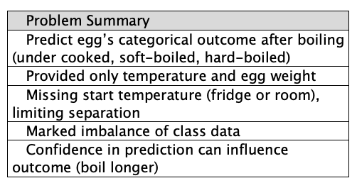
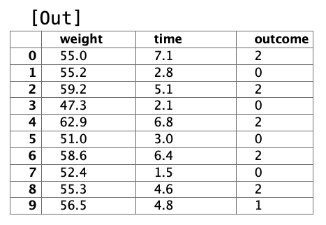
The data is from an experiment in egg boiling. The boil durations are provided along with the egg’s weight in grams and the finding on cutting it open. Findings are categorised into one of three classes: under cooked, soft-boiled and hard-boiled. We want the egg’s outcome from its weight and boiling time. The problem is insanely simple, so much so that the data is near being linearly separable¹. But not quite, as the egg’s pre-boil life (fridge temperature or cupboard storage at room temperature) aren’t provided and as you’ll see this swings cooking times. Without the missing data we can’t be certain what we’ll find when opening an egg up. Knowing how certain we are we can influence the outcome here as we can with most problems. In this case if relatively confident an egg’s undercooked we’ll cook it more before cracking it open.
数据来自煮鸡蛋的实验。 提供煮沸的时间以及鸡蛋的重量(克)和切开鸡蛋的发现。 调查结果分为以下三类之一:未煮熟,软煮和硬煮。 我们想要鸡蛋的重量和煮沸时间来获得结果。 这个问题非常简单,以至于数据几乎可以线性分离。 但事实并非如此,因为没有提供鸡蛋的预煮寿命(冰箱温度或橱柜在室温下存储),并且您会看到这会改变烹饪时间。 没有缺少的数据,我们将无法确定打开鸡蛋时会发现什么。 知道自己的确定性,我们可以像对待大多数问题一样在这里影响结果。 在这种情况下,如果对鸡蛋未完全煮熟有相对的把握,我们会在将其打开之前将其煮熟。
Let’s have a look at the data first to see what we’re dealing with. If you want to feel the difference for yourself you can get the data at github.com/DoctorLoop/BayesianDeepLearning/blob/master/egg_times.csv. You’ll need Pandas and Matplotlib for exploring the data. (pip install — upgrade pandas matplotlib) Download the dataset to the same directory you’re working from. From a Jupyter notebook type pwd on its own in a cell to find out where that directory is if unsure.
首先让我们看一下数据,看看我们正在处理什么。 如果您想自己感觉与众不同,可以在github.com/DoctorLoop/BayesianDeepLearning/blob/master/egg_times.csv上获取数据。 您将需要Pandas和Matplotlib来浏览数据。 (pip安装-升级pandas matplotlib)将数据集下载到您正在使用的目录中。 在Jupyter笔记本中,在一个单元格中单独键入pwd,以查明该目录在哪里(如果不确定)。
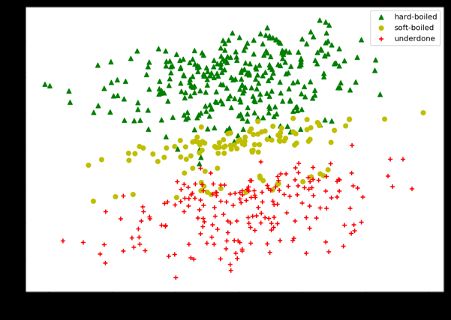
https://gist.github.com/DoctorLoop/5a8633691f912d403e04a663fe02e6aa https://gist.github.com/DoctorLoop/5a8633691f912d403e04a663fe02e6aa https://gist.github.com/DoctorLoop/21e30bdf16d1f88830666793f0080c63 https://gist.github.com/DoctorLoop/21e30bdf16d1f88830666793f0080c63 Figure 2.01 Scatter plot of egg outcomes 图2.01鸡蛋结果散布图And let’s see it now as a histogram.
现在让我们将其视为直方图。
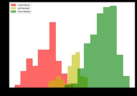
https://gist.github.com/DoctorLoop/2a5e95a68a29315f167e0e875e7fae16 https://gist.github.com/DoctorLoop/2a5e95a68a29315f167e0e875e7fae16 Figure 2.02 Histogram of egg times by outcome 图2.02按结果划分的鸡蛋时间直方图It seems I wasn’t so good at getting my eggs soft-boiled as I like them so we see a fairly large class imbalance with twice as many underdone instances and three times as many hardboiled instances relative to the soft-boiled lovelies. This class imbalance can spell trouble for conventional neural networks causing them to underperform and an imbalanced class size is a common finding.
看来我不太喜欢自己煮鸡蛋,因此我们发现班级失衡相当大,相对于煮熟的熟食来说,欠缺实例的数量是未煮熟实例的两倍,硬煮实例的数量是三倍。 这种类别的不平衡会给常规神经网络带来麻烦,导致它们表现不佳,并且类别规模的不平衡是常见的发现。
Note that we’re not setting density to True (False is the default so doesn’t need to be specified) as we’re interested in comparing actual numbers. While if we were comparing probabilities sampled from one of the three random variables, we’d want to set density=True to normalise the histogram summing the data to 1.0.
请注意,我们没有将密度设置为True(默认值为False,因此无需指定),因为我们希望比较实际数字。 如果要比较从三个随机变量之一中采样的概率,则需要设置density = True以将直方图归一化以将数据求和为1.0。
Histograms can be troublesome for discretisation of data as we need explicitly specify (or use an algorithm to specify for us) the number of bins to gather values by. Bin size vastly influences how the data appears. As an alternative we can opt to use a kernel density estimate, but it’s often nice when comparing groups as we are here to use a violin plot instead. A violin plot is a hybrid with a box plot showing the smoothed distribution for easy comparison. In python it’s both easier and prettier to do violin plots with the Seaborn library (pip install — upgrade seaborn). But I’ll show it here in matplotlib to be consistent.
直方图对于数据离散化可能很麻烦,因为我们需要明确指定(或使用算法为我们指定)收集值所依据的仓数。 容器大小极大地影响了数据的显示方式。 作为替代方案,我们可以选择使用核密度估计,但是在比较组时通常很好,因为这里我们改用小提琴图。 小提琴图是带盒图的混合图,它显示了平滑的分布以便于比较。 在python中,使用Seaborn库(小提琴安装-升级seaborn)进行小提琴绘图既简单又美观。 但是我将在matplotlib中展示它以保持一致。
https://gist.github.com/DoctorLoop/c5bac12d7b7ebd7758cc83f0fe931fc0 https://gist.github.com/DoctorLoop/c5bac12d7b7ebd7758cc83f0fe931fc0 Figure 2.03 Violin plot of egg times by outcome. Central bar indicates mean. 图2.03小提琴将鸡蛋乘以时间的结果图。 中心栏表示平均值。Alright great. Now let’s highlight the architectural differences between neural networks we’re actually here to learn about. We’ll implement a classical dense architecture first then transform it into a powerful Bayesianesque equivalent. We implement the dense model with the base library (either TensorFlow or Pytorch) then we use the add on (TensorFlow-Probability or Pyro) to create the Bayesian version. Unfortunately the code for TensorFlow’s implementation of a dense neural network is very different to that of Pytorch so go to the section for the library you want to use.
很好。 现在让我们重点介绍我们实际上要学习的神经网络之间的架构差异。 我们将首先实现经典的密集架构,然后将其转换为功能强大的贝叶斯风格。 我们使用基础库(TensorFlow或Pytorch)实现密集模型,然后使用添加项(TensorFlow-Probability或Pyro)创建贝叶斯版本。 不幸的是,用于TensorFlow的密集神经网络实现的代码与Pytorch的代码非常不同,因此请转到要使用的库部分。
TensorFlow / TensorFlow概率 (TensorFlow/TensorFlow-Probability)
The source code is available at
源代码位于
github.com/DoctorLoop/BayesianDeepLearning/
github.com/DoctorLoop/BayesianDeepLearning/
https://gist.github.com/DoctorLoop/3a67fd1197a355f68f45076be0074844 https://gist.github.com/DoctorLoop/3a67fd1197a355f68f45076be0074844We’re using Keras for the implementation as it’s what we need for our later TFP model. We start training by calling the compiled model as shown bellow.
我们正在使用Keras进行实施,因为这是我们以后的TFP模型所需要的。 我们通过调用如下所示的编译模型开始训练。
https://gist.github.com/DoctorLoop/f6c74509046068ae7ac37efe00d08545 https://gist.github.com/DoctorLoop/f6c74509046068ae7ac37efe00d08545You’ll see TensorBoard is used to keep a record of our training — It’s good to take advantage of TensorBoard as its powerful means of model debugging and one of the key features of TensorFlow. If we want to output training progress beneath the cell during training we can use the Keras output with the verbose parameter of model.fit set to 1. The problem with the Keras output is it’ll print the loss for every epoch. Here we’re training for 800 epochs so we’ll get a long a messy output. It’s therefore nicer to create a custom logger giving control over the frequency of printing the loss. The source code for the custom logger is very simple and available in the notebook at Github. Both the TensorBoard callback (and any custom logger) is passed to the callbacks parameter but this can be ignored if you don’t want to just log every epoch in the notebook. The great thing about Keras is it’ll split the data for validation for us and saving time. Here 10% of the data is used for validation. Some people use 25% of the data for validation but as data is the most important consideration for a neural network and the datasets tend to be fairly large 10% works fine and gives the model a better chance of reaching our training goals. The Github notebook also shows how to use class weights to address the class imbalance we discussed earlier. Finally, ensure validation is infrequent if training time is important as validation is considerably slower than the training itself (especially with a custom logger where approx 10x slower) therefore making training longer.
您会看到TensorBoard用于记录我们的培训-很好地利用TensorBoard作为其强大的模型调试工具和TensorFlow的关键功能之一。 如果我们想在训练过程中在单元下方输出训练进度,我们可以将Keras输出与model.fit的详细参数一起使用,设置为1。Keras输出的问题是它将打印每个时期的损失。 在这里,我们正在训练800个纪元,因此我们会得到很长的混乱输出。 因此,最好是创建一个自定义记录器,以控制打印损失的频率。 自定义记录器的源代码非常简单,可以在Github的笔记本中找到。 TensorBoard回调(以及任何自定义记录器)都传递给callbacks参数,但是如果您不想只记录笔记本中的每个纪元,则可以忽略该参数。 Keras的妙处在于它将拆分数据以供我们验证并节省时间。 这里有10%的数据用于验证。 有些人使用25%的数据进行验证,但由于数据是神经网络最重要的考虑因素,而数据集往往相当大,因此10%的数据可以很好地工作,并使模型有更好的机会达到我们的训练目标。 Github笔记本还显示了如何使用类权重来解决我们前面讨论的类不平衡问题。 最后,如果培训时间很重要,请确保不经常进行验证,因为验证比培训本身要慢得多(尤其是使用自定义记录器,速度大约慢10倍),因此会使培训时间更长。
Final loss is around 0.15 with an accuracy of 0.85. If you train for more than 800 epochs after epoch 1200 you’ll see validation accuracy decreasing even though loss is still declining. That’s because we’ve started to overfit to the training data. When we’re overfitting we’re making our model depend on the specific training instances meaning it doesn’t generalise well to our unseen validation data or the intended real-world application of the model². Overfitting is the bane of conventional neural networks that often need large datasets and early stopping approaches to mitigate.
最终损失约为0.15,准确度为0.85。 如果您在1200期之后进行了800多个培训,那么即使损失仍在减少,验证准确性也会下降。 这是因为我们已经开始过度拟合训练数据。 当我们过度拟合时,我们将模型建立在特定的训练实例上,这意味着它不能很好地推广到我们看不见的验证数据或模型的预期实际应用中²。 过度拟合是传统神经网络的祸根,传统神经网络通常需要大型数据集和早期停止方法来缓解。
But we’re here to learn about solutions not problems! Enter stage our Bayesian neural networks which are resistant to overfitting, aren’t particularly bothered about class imbalance and most importantly perform extraordinarily well with very little data.
但是,我们在这里了解解决方案而不是问题! 进入我们的抵抗过度拟合的贝叶斯神经网络,对于类的不平衡并不会特别打扰,最重要的是, 在数据很少的情况下,它表现出色 。
Let’s take a look at a Bayesian implementation of the model.
让我们看一下该模型的贝叶斯实现。
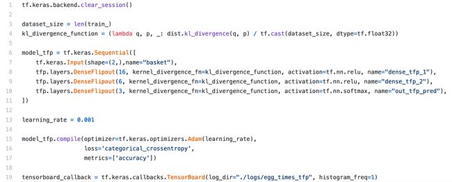
https://gist.github.com/DoctorLoop/f00c18f591553685e06a79fdbe4b68e0 https://gist.github.com/DoctorLoop/f00c18f591553685e06a79fdbe4b68e0It’s very similar to our conventional model except we’re using a flipout layer from TensorFlow-Probability instead. We specify a kernel divergence function which is the Kullback-Leibler divergence mentioned earlier. That’s about it.
它与我们的常规模型非常相似,只不过我们使用的是TensorFlow-Probability中的翻转层。 我们指定一个内核散度函数,它是前面提到的Kullback-Leibler散度。 就是这样
火炬/火 (Pytorch/Pyro)
When comparing a conventional dense model to a Bayesian equivalent Pyro does things differently. With Pyro we always create a conventional model first then upgrade it by adding two new functions to make the conversion. The conventional model is needed to provide a way to automatically sample values from the weight distributions. The sampled values are plugged into the corresponding position on the conventional model to produce an estimate of training progress. You’ll remember from the last chapter how training conditions (trains) the weight distributions. In clear speech it means training shifts the normal distributions and alters their scale to represent each weight. However to make a prediction we still plug in solid single-weight values. While we can’t use the distributions wholesale to make predictions we can take many predictions each with different sampled weight values to approximate the distribution. That’s where the dense model we first build fits in nicely.
当将传统的稠密模型与贝叶斯等效的Pyro进行比较时,事情会有所不同。 使用Pyro,我们总是先创建一个常规模型,然后通过添加两个新功能进行转换来升级它。 需要传统模型来提供一种从重量分布中自动采样值的方法。 采样值被插入到常规模型的相应位置,以生成训练进度的估计值。 您将从上一章中还记得训练条件 (训练)如何分配体重。 用清晰的言语意味着训练会改变正态分布并改变其比例以表示每个权重。 但是,为了做出预测,我们仍然插入固定的单权重值。 尽管我们不能使用分布批发来进行预测,但我们可以采用许多预测,每个预测具有不同的采样权重值来近似分布。 这就是我们最初构建的密集模型的完美体现。
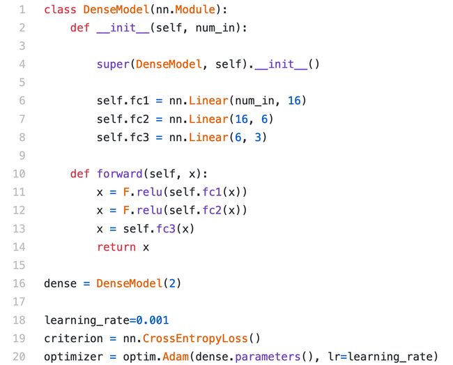
We’ll start then with a class to enclose our dense model. The full source code is available in an online notebook at https://github.com/DoctorLoop/BayesianDeepLearning.
然后,我们从一个类开始以封装我们的密集模型。 完整的源代码可在https://github.com/DoctorLoop/BayesianDeepLearning的在线笔记本中找到。
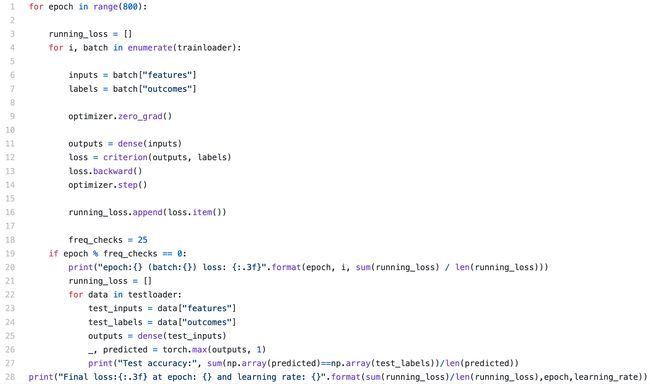
https://gist.github.com/DoctorLoop/33b192030388c46d0a2591459b2f6623 https://gist.github.com/DoctorLoop/33b192030388c46d0a2591459b2f6623We’ve setup three layers with only the first two layers utilising an activation function. Then we’ve specified our loss function and optimizer. Be careful to note that for this model we’re utilising the torch.optim.Adam (Pytorch optimizer) rather than the Pyro optimizer. If you try to use Pyro here it’ll throw errors as the parameters are presented differently. Our training loop isn’t anything special if you’ve used Pytorch before. 800 epochs are perfectly excessive, but so what.
我们使用激活功能设置了三层,只有前两层。 然后,我们指定了损失函数和优化器。 请注意,对于此模型,我们使用的是torch.optim.Adam(Pytorch优化器),而不是Pyro优化器。 如果您在此处尝试使用Pyro,由于参数显示方式不同,将会引发错误。 如果您以前使用过Pytorch,我们的培训循环就没什么特别的了。 800个纪元是完全多余的,但那又如何呢?
https://gist.github.com/DoctorLoop/75854f26bee106d9b596b2ee0544c5d5 https://gist.github.com/DoctorLoop/75854f26bee106d9b596b2ee0544c5d5[Out]:
…
Test accuracy: 0.88
Final loss:0.173 at epoch: 799 and learning rate: 0.001Pretty good performance here and quick too. If you’re new to Pytorch and have experience elsewhere you might wonder at the lack of softmax. In Pytorch it’s important to note softmax is built into CrossEntropyLoss.
这里的表现相当不错,而且速度也很快。 如果您是Pytorch的新手,并且在其他地方有经验,那么您可能会怀疑缺少softmax。 在Pytorch中,需要注意的是softmax是内置在CrossEntropyLoss中的。
Let’s get on with upgrading it. Here are the two new functions I mentioned, the model and guide.
让我们继续进行升级。 这是我提到的两个新功能,即模型和指南。
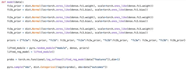
https://gist.github.com/DoctorLoop/a4dcf6b0f7f1ece43087534ebdfcaa08 https://gist.github.com/DoctorLoop/a4dcf6b0f7f1ece43087534ebdfcaa08We will save intricate discussion about what these function do to another article in the series. Simply put, the model explicitly declares the distributions used for each layer to replace the point values. While the guide declares the variables used to condition (train) those distributions. You’ll notice the functions look similar but on close inspection the model lists the individual distributions for weights and for biases then the guide lists the distributions for the mean and sigma for every weight and bias distribution in the model. That sounds a bit meta — because it is. Save pondering it until later and just have a feel for the training now³.
我们将把关于这些功能的复杂讨论保存到本系列的另一篇文章中。 简而言之,模型明确声明了用于每一层的分布以替换点值。 虽然指南声明了用于条件(训练)这些分布的变量。 您会注意到功能看起来很相似,但仔细检查后,模型会列出权重和偏差的单个分布,然后指南会列出模型中每个权重和偏差分布的均值和sigma 的分布 。 这听起来有点元-因为是。 无需再考虑,直到以后再去体验一下。³
https://gist.github.com/DoctorLoop/5a3837c384181b391df5927bdd5e2ab5 https://gist.github.com/DoctorLoop/5a3837c384181b391df5927bdd5e2ab5Training this beautiful monster is fast. We arrive at an accuracy slightly higher than the dense model 0.88–0.90 with a loss of 0.18. I’ve implemented a few extra functions here to make training easier (the trainloader and a predict function) and provide the full source in the GitHub notebook.
训练这个美丽的怪物很快。 我们得出的精度略高于密集模型0.88–0.90,损失为0.18。 我在这里实现了一些额外的功能,以简化培训(trainloader和预测功能),并在GitHub笔记本中提供完整的源代码。
贝叶斯深度学习的损失函数 (Loss function for Bayesian deep learning)
We can’t backpropagate through random variables (because by definition they’re random). Therefore we cheat and reparametrize the very distributions and have training update distribution parameters. With this fundamental change we need a different way to calculate training loss.
我们无法通过随机变量向后传播(因为根据定义,它们是随机的)。 因此,我们欺骗并重新参数化了非常分布,并具有训练更新分布参数。 有了这一根本性的改变,我们需要一种不同的方法来计算训练损失。
You may have already known of negative log likelihood that’s used in conventional models. It reflects the probability the data was generated by the model. Don’t worry about what this means now. Instead know that we approximate this loss by taking the average of a large number of samples. But along with our negative log likelihood we combine a new loss leveraging the distribution under calculation. The new loss is Kullback–Leibler divergence (KL divergence) and provides a measure of how different two distributions are from each other. We’ll refer to KL divergence frequently and find it useful in other areas including metrics of uncertainty⁴. Negative log likelihood is added to the KL divergence to get ELBO loss (expected lower bound on margin likelihood, also known as variational free energy). ELBO loss allows us to approximate distributions during training and benefit hugely in terms of trainability and training time.
您可能已经知道传统模型中使用的对数可能性为负。 它反映了模型生成数据的可能性。 现在不用担心这意味着什么。 相反,要知道我们通过取大量样本的平均值来近似估算此损失。 但是,除了负对数可能性外,我们还利用计算中的分布组合了新的损失。 新的损失是Kullback-Leibler散度(KL散度),它提供了两种分布之间的差异程度的度量。 我们将经常提及KL分歧,并发现它在其他领域(包括不确定性指标⁴)很有用。 将负对数似然率添加到KL散度中以获得ELBO损失(预期的裕度似然性下限,也称为变异自由能)。 ELBO损失使我们能够在训练过程中近似地分配分布,并在可训练性和训练时间方面受益匪浅。
Finally, to conclude, let’s glimpse what happens when we make predictions, after all it’s what we’re here for.
最后,总而言之,让我们瞥见进行预测时会发生什么,毕竟这是我们的目标。
https://gist.github.com/DoctorLoop/41c31bf30339dc1b4b4c7e69a001b9bf https://gist.github.com/DoctorLoop/41c31bf30339dc1b4b4c7e69a001b9bfWe make 5000 samples (this can take a few minutes depending on your computer). With a conventional neural network all these predictions would be exactly the same so it would be a pointless endeavour. But we aren’t using conventional neural networks anymore.
我们制作了5000个样本(这可能需要几分钟的时间,具体取决于您的计算机)。 使用传统的神经网络,所有这些预测将完全相同,因此这将是毫无意义的尝试。 但是我们不再使用传统的神经网络了。
https://gist.github.com/DoctorLoop/1ae0d213d3875dd569d582c810769fc7 https://gist.github.com/DoctorLoop/1ae0d213d3875dd569d582c810769fc7 Figure 2.04: Histograms of 5000 samples for 3 test inputs 图2.04: 3个测试输入的5000个样本的直方图The predict function samples multiple different model versions from the master model we trained with TFP or Pyro. The three test instances we’ve input each result in well defined peaks. The first test instance (red histogram) had a weight of 61.2g and a boiling time of 4.8minutes. Most the time we can see our model predicted it would be a soft-boiled egg, 5% of the time however it predicted an underdone egg and 2% of the time it thought it would be a hard-boiled egg. The model is reasonably confident in this prediction but not as confident as the second test example (green histogram) which almost always predicts a hardboiled result for a 53g egg boiled for 6minutes. How do we achieve consistency from the model if predictions are different each time? We just take the average. If predictions are too variable, i.e. a third in each class we’d not want to make a prediction, except we can act on the information and tell the user that the model is uncertain about the outcome (or ask ourselves if we need work on the model/data some more!) In both cases we gain really powerful information about something a conventional model can’t offer. We can therefore think of a conventional model as always arrogant while our new model is appropriate. It’s cautious, but confident when confidence is correct. We don’t need be a computer-science psychologist to appreciate the preferable model-personality.
预测函数从我们使用TFP或Pyro训练的主模型中采样了多个不同的模型版本。 我们输入的三个测试实例的每个结果均定义良好的峰。 第一个测试实例(红色直方图)的重量为61.2g,沸腾时间为4.8分钟。 在大多数时候,我们可以看到我们的模型预测它是一个煮熟的鸡蛋,但有5%的时间预测它是一个煮熟的鸡蛋,而有2%的时间则认为它是一个煮熟的鸡蛋。 该模型对该预测相当有信心,但不如第二个测试示例(绿色直方图)那么有信心,第二个测试示例几乎总是可以预测53分钟煮沸6分钟的鸡蛋的煮熟结果。 如果每次预测都不同,我们如何从模型中获得一致性? 我们只取平均值。 如果预测变量太大,即每个类别中的三分之一,我们都不想做出预测,除非我们可以根据信息采取行动,并告诉用户该模型对结果不确定(或者问自己是否需要开展工作)模型/数据更多!)在两种情况下,我们都能获得有关常规模型无法提供的强大信息。 因此,我们可以认为传统模型总是傲慢自大,而我们的新模型却是合适的。 这是谨慎的,但在信心正确的时候要有信心。 我们不需要成为计算机科学心理学家就可以欣赏可取的模型个性。
摘要 (Summary)
In this chapter we’ve explored the changes in a basic Bayesian model and seen some major advantages accompanying it. We’ve seen how to do this in TensorFlow-Probability and in Pyro. While the model is fully functional, at this stage it isn’t perfect and neither is it truly Bayesian. Whether a ‘truer’ model matters depends on your circumstances. In subsequent articles we’ll include discussion about imperfections like the use of softmax and how we can address them. In the next article our main focus will be on image prediction with Bayesian convolutional deep learning. If my writing looked a little more formal I’d perhaps be more confident of seeing you there!
在本章中,我们探讨了基本贝叶斯模型的变化,并看到了一些伴随它的主要优点。 我们已经在TensorFlow-Probability和Pyro中看到了如何执行此操作。 尽管该模型具有完整的功能,但在现阶段还不是很完美,也不是真正的贝叶斯模型。 “特鲁尔”模型是否重要取决于您的情况。 在随后的文章中,我们将讨论关于诸如softmax的使用之类的缺陷以及如何解决这些缺陷。 在下一篇文章中,我们的主要焦点将是利用贝叶斯卷积深度学习进行图像预测。 如果我的作品看起来更正式一点,我也许会更有信心在那见到你!
1 Therefore it’s somewhat of an abuse to solve the problem with a neural network when simpler models would do fine.
1因此,当较简单的模型可以解决问题时,使用神经网络解决问题有点滥用。
2 Unsure what the real-world application is here, a breakfast cafe?
2不确定早餐咖啡馆是这里的真实应用程序吗?
3 If your thinking: Wow the TensorFlow-Probability code looked way simpler it’s because it does the operations for you for now. That said, we can make the Pyro code simpler as well by using a Pyro autoguide. As it suggests this plays the role of the guide for you. But we’re here to learn the wonder of Bayesian deep learning so we need to get exposure at some point!
3如果您的想法:哇,TensorFlow-Probability代码看起来更简单了,因为它现在为您执行操作。 也就是说,我们可以使用Pyro自动向导来简化Pyro代码。 正如它所暗示的那样,它为您扮演了指南的角色。 但是我们在这里要学习贝叶斯深度学习的奇迹,因此我们需要在某个时候获得曝光!
4 Interestingly we can make a simple classifier with reasonable performance by using KL divergence directly, i.e. an image pattern classifier can be built with the local binary pattern algorithm and KL. In this partnership KL compares the distributions of corners and edges between the input image and an image with a known pattern.
4有趣的是,我们可以直接使用KL散度来制作一个具有合理性能的简单分类器,即可以使用局部二进制模式算法和KL构建图像模式分类器。 在这种伙伴关系中,KL比较输入图像和具有已知图案的图像之间的角和边缘分布。
翻译自: https://towardsdatascience.com/bayesian-neural-networks-2-fully-connected-in-tensorflow-and-pytorch-7bf65fb4697
pytorch贝叶斯网络
