无监督学习 k-means
有关深层学习的FAU讲义 (FAU LECTURE NOTES ON DEEP LEARNING)
These are the lecture notes for FAU’s YouTube Lecture “Deep Learning”. This is a full transcript of the lecture video & matching slides. We hope, you enjoy this as much as the videos. Of course, this transcript was created with deep learning techniques largely automatically and only minor manual modifications were performed. Try it yourself! If you spot mistakes, please let us know!
这些是FAU YouTube讲座“ 深度学习 ”的 讲义 。 这是演讲视频和匹配幻灯片的完整记录。 我们希望您喜欢这些视频。 当然,此成绩单是使用深度学习技术自动创建的,并且仅进行了较小的手动修改。 自己尝试! 如果发现错误,请告诉我们!
导航 (Navigation)
Previous Lecture / Watch this Video / Top Level / Next Lecture
上一个讲座 / 观看此视频 / 顶级 / 下一个讲座
Welcome back to deep learning! Today, we want to continue talking about unsupervised methods and look into a very popular technique that is the so-called autoencoder.
欢迎回到深度学习! 今天,我们要继续谈论无监督方法,并研究一种非常流行的技术,即所谓的自动编码器。
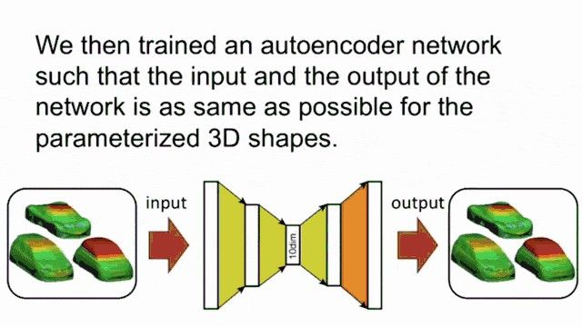
An example for “auto”-encoding shapes (pun intended). Image created using gifify. Source: YouTube 一个“自动”编码形状的示例(用于双关语)。 使用 gifify创建的 图像 。 资料来源: YouTubeSo, here are our slides. Part two of our lecture and the topic autoencoders. Well, the concept of the autoencoder is that we want to use the ideas of feed-forward neural networks. You could say that a feed-forward neural network is a function of xthat produces some encoding y.
所以,这是我们的幻灯片。 我们的讲座的第二部分和主题自动编码器。 好吧,自动编码器的概念是我们要使用前馈神经网络的思想。 您可以说前馈神经网络是x的函数,它产生一些编码y 。
CC BY 4.0 from the 深度学习讲座中 Deep Learning Lecture. CC BY 4.0下的图像。Now, the problem is: “How can we generate a loss in such a constellation?” The idea is rather simple. We add an additional layer here on top and the purpose of the layer is to compute decoding. So, we have another layer that is g(y). g(y) produces some x hat. The loss that we can then define is that x hat and x need to be the same. So the autoencoder tries to learn an approximation of the identity. Well, that sounds rather simple. To be honest, if we have exactly the same number of nodes in the input and in the hidden layer for y here, then the easiest solution would probably be the identity. So why is this useful at all?
现在的问题是:“我们如何在这样的星座中产生损失?” 这个想法很简单。 我们在此处添加一个附加层,该层的目的是计算解码。 因此,我们还有另一个层g( y )。 g( y )产生一些x帽。 我们可以定义的损失是x hat和x必须相同。 因此,自动编码器尝试了解身份的近似值。 好吧,听起来很简单。 老实说,如果我们在输入中和在y的隐藏层中具有完全相同数量的节点,那么最简单的解决方案可能就是身份。 那么,这到底为什么有用呢?
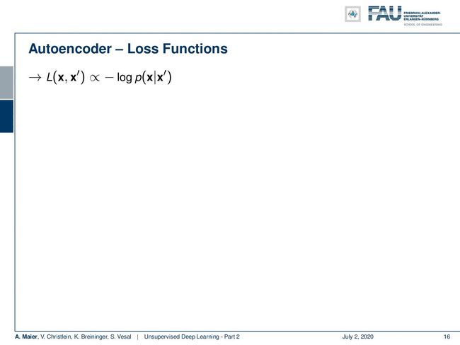
CC BY 4.0 from the 深度学习讲座中 Deep Learning Lecture. CC BY 4.0下的图像。Well, let’s look at some loss functions. What you can typically use is a loss function that then operates here on x and some x’. It can be proportional to a negative log-likelihood function where you have p(x|x’) and resulting functions. Then, in a similar way, as we’ve seen earlier in this class, you can use the squared L2 norm where you assume your probability density of a function to be a normal distribution with uniform variance. Then, you end up with the L2 loss. It is simply xminus x’ and this encapsulated in an L2 norm. Of course, you can also do things like cross-entropy. So, if you assume the Bernoulli distribution, you see that we end up exactly with our cross-entropy. This is simply the sum over the weighted xtimes the logarithm of x’ subscript i plus 1-x subscript i times the logarithm of 1 — x’ subscript i. Remember that if you want to use it this way, then your x’s need to be in the range of probabilities. So, if you want to apply this kind of loss function, then you may want to use it in combination with a softmax function.
好吧,让我们看一些损失函数。 通常可以使用的是损失函数,然后在此处对x和某些x '进行运算。 它可以与负对数似然函数成比例,其中您有p( x | x ')和所得函数。 然后,以类似的方式,就像我们在本课程前面所看到的那样 ,您可以使用平方L2范数,在此假设函数的概率密度为具有均方差的正态分布。 然后,您最终会遭受L2损失。 它就是x减去x ',并封装在L2范数中。 当然,您也可以做交叉熵之类的事情。 因此,如果您假设伯努利分布,您会发现我们恰好以交叉熵结束。 这仅是加权x乘以x '下标i的对数加上1- x下标i乘以1 — x '下标i的对数的总和。 请记住,如果您想以这种方式使用它,则x必须在概率范围内。 因此,如果您想应用这种损失函数,则可能希望将其与softmax函数结合使用。
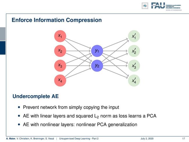
CC BY 4.0 from the 深度学习讲座中 Deep Learning Lecture. CC BY 4.0下的图像。Ok, so here are some typical strategies to construct such autoencoders. I think one of the most popular ones is the undercomplete autoencoder. So here, you enforce information compression by using fewer neurons in the hidden layer. You try to find a transform that does essentially a dimensionality reduction to the hidden layer. Then, you try to expand from this hidden layer onto the original data domain and try to find a solution that produces a minimum loss. So, you try to learn compression here. By the way, if you do this with linear layers and squared L2 norm, you essentially learn a principal component analysis (PCA). If you use it with nonlinear layers, you end up with something like a nonlinear PCA generalization.
好的,这是构造此类自动编码器的一些典型策略。 我认为最流行的一种是不完整的自动编码器。 因此,在这里,您可以通过在隐藏层中使用较少的神经元来实施信息压缩。 您尝试找到一种实质上减少了隐藏层维数的变换。 然后,您尝试从该隐藏层扩展到原始数据域,并尝试找到产生最小损失的解决方案。 因此,您尝试在此处学习压缩。 顺便说一句,如果您使用线性层和平方L2范数执行此操作,则实际上您将学习主成分分析(PCA)。 如果将其与非线性层一起使用,则最终会出现类似非线性PCA泛化的情况。
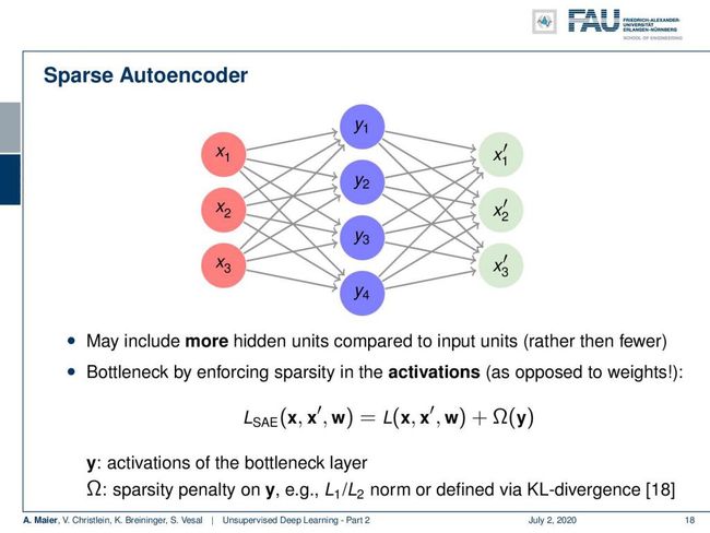
CC BY 4.0 from the 深度学习讲座中 Deep Learning Lecture. CC BY 4.0下的图像。There are also things like these sparse autoencoders. Here, we have a different idea. We even increase the number of neurons, to resemble a one-hot encoded vector. So, you may say: “Why would you increase the number of your neurons? Then, you could even find a much simpler solution like the identity and neglect a couple of those neurons!” So, this idea will not work straightforwardly. You have to enforce sparsity which is also coining the name sparse autoencoder. Here, you have to enforce sparsity in the activations using some additional regularization. For example, you can do this with an L1 norm on the activations in y. Remember, the sparsity in the sparse autoencoder stems from sparsity in the activations, not from sparsity in the weights. If you look at your identity, then you see this is simply a diagonal matrix with ones on the diagonal. So, this would also be a very sparse solution. So, again enforce the sparsity on the activations, not on the weights.
也有类似这些稀疏自动编码器的东西。 在这里,我们有一个不同的想法。 我们甚至增加了神经元的数量,类似于一个热编码的载体。 因此,您可能会说:“为什么要增加神经元的数量? 然后,您甚至可以找到一种更简单的解决方案,例如身份验证,而忽略其中的两个神经元!” 因此,这个想法不会直接起作用。 您必须实施稀疏性,这也造就了稀疏自动编码器的名称。 在这里,您必须使用一些其他正则化方法来强制激活稀疏性。 例如,您可以对y中的激活使用L1范数来执行此操作。 请记住,稀疏自动编码器中的稀疏性源自激活中的稀疏性,而不是权重中的稀疏性。 如果您看一下自己的身份,那么您会看到这只是一个对角矩阵,对角线上有一个。 因此,这也是一个非常稀疏的解决方案。 因此,再次对激活而不是权重实施稀疏性。
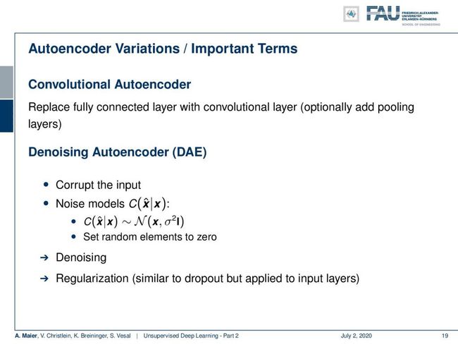
Sparse autoencoding in action. Image created using gifify. Source: YouTube 有效的稀疏自动编码。 使用 gifify创建的 图像 。 资料来源: YouTubeWhat else can be done? Well, you can use autoencoder variations. You can combine it essentially with all the recipes we’ve learned so far in this class. You can build convolutional autoencoders. There, you replace the fully connected layers with convolutional layers and you can optionally also add pooling layers.
还有什么可以做的? 好吧,您可以使用自动编码器变体。 您可以将它与我们在课堂上到目前为止学到的所有食谱结合起来。 您可以构建卷积自动编码器。 在那里,您可以用卷积层替换完全连接的层,还可以选择添加池化层。
CC BY 4.0 from the 深度学习讲座中 Deep Learning Lecture. CC BY 4.0下的图像。There is the denoising autoencoder which is also a very interesting concept. There you corrupt the input with noise and the target is then the noise-free original sample. So, this then results in a trained system that does not just do dimensionality reduction or finding a sparse representation. At the same time, it also performs denoising and you could argue that this is an additional regularization that is similar to dropout but essentially applied to the input layers. There’s also a very interesting paper called noise2noise where they show that you can even build such denoising auto-encoders even if you have a noisy target. The key here then is that you have a different noise pattern in the input and in the target and this way you can also train a denoising autoencoder at least if you build on top of convolutional autoencoders.
有降噪自动编码器,这也是一个非常有趣的概念。 在那里,您会用噪声破坏输入,然后目标就是无噪声的原始样本。 因此,这导致了一个训练有素的系统,该系统不仅减少了维数或发现了稀疏表示。 同时,它还会执行去噪,您可能会说这是一个附加的正则化,类似于丢包,但实际上应用于输入层。 还有一篇非常有趣的论文,称为noise2noise ,它们表明即使您有嘈杂的目标,您也可以构建这种去噪自动编码器。 然后,这里的关键是您在输入和目标中具有不同的噪声模式,并且至少在基于卷积自动编码器的情况下,这种方式也可以训练去噪自动编码器。
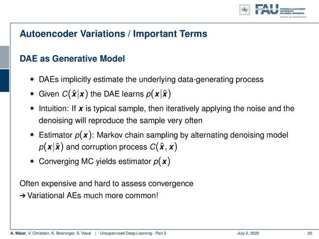
CC BY 4.0 from the 深度学习讲座中 Deep Learning Lecture. CC BY 4.0下的图像。Now, you can even go as far as using the denoising autoencoder as a generative model. The idea here is that if you sample your corruption model, your noise model frequently. Then, the denoising autoencoder learns the probability of the respective input. So, if you have x as a typical sample, then by iteratively applying the noise and the denoising will reproduce this sample very often. So, you can then use a Markov chain and you alternate the denoising model and the corruption process. This then leads to an estimator of p(x). To be honest, this is often expensive and it’s very hard to assess the convergence which is the reason why so-called variational autoencoders are much more common. We will talk about those variational autoencoders in a couple of slides.
现在,您甚至可以将去噪自动编码器用作生成模型。 这里的想法是,如果您对损坏模型进行采样,那么您的噪声模型就会频繁出现。 然后,去噪自动编码器学习各个输入的概率。 因此,如果您将x作为典型样本,则通过迭代应用噪声和去噪将非常频繁地重现该样本。 因此,您可以使用马尔可夫链,然后交替使用降噪模型和破坏过程。 然后,这导致了p( x )的估计。 老实说,这通常很昂贵,并且很难评估收敛性,这就是所谓的变分自动编码器更为普遍的原因。 我们将在几张幻灯片中讨论那些可变自动编码器。
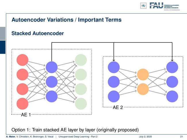
CC BY 4.0 from the 深度学习讲座中 Deep Learning Lecture. CC BY 4.0下的图像。There are some variations that we need to introduce first. There’s the so-called stacked autoencoder. In the stacked autoencoder, you essentially put an autoencoder inside of an autoencoder. This allows us to build essentially deep autoencoders. We see this here in the concept. Autoencoder 1 is using in the hidden layer the Autoencoder 2 which is indicated by the blue nodes. You can stack those into a single autoencoder.
首先需要引入一些变体。 有所谓的堆叠式自动编码器。 在堆叠式自动编码器中,您实际上是将自动编码器放在自动编码器内部。 这使我们能够构建本质上很深的自动编码器。 我们在概念中看到了这一点。 自动编码器1在隐藏层中使用由蓝色节点表示的自动编码器2。 您可以将它们堆叠到单个自动编码器中。
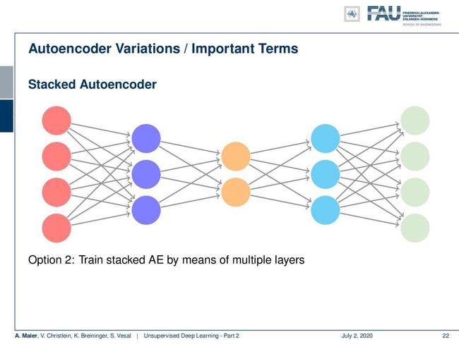
CC BY 4.0 from the 深度学习讲座中 Deep Learning Lecture. CC BY 4.0下的图像。This gives rise to the following model and then the idea is to have a gradual dimensionality reduction. You already have guessed this: this is also something that is very commonly used together with convolutions and pooling.
这产生了以下模型,然后的想法是逐步减小维数。 您已经猜到了:这也是卷积和池化一起非常常用的东西。
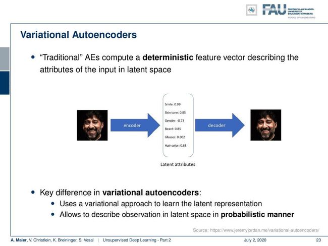
CC BY 4.0 from the 深度学习讲座中 Deep Learning Lecture. CC BY 4.0下的图像。Now let’s go into the concept of the variational autoencoders. This is a bit of a different concept. In the traditional autoencoders, you try to compute a deterministic feature vector that describes the attributes of the input in some kind of latent space. So let’s say, you had a latent space that characterizes different features, for example, of a face. Then, you could argue that this encoder then takes the image and projects it onto some probably unknown latent attributes. Here, we give them some additional interpretation. So for every attribute, you have a certain score and from the score then you generate the original image again. The key difference in variational auto-encoders is that you use a variational approach to learn the latent representation. It allows you to describe the latent space in a probabilistic manner.
现在让我们进入变分自动编码器的概念。 这有点不同。 在传统的自动编码器中,您尝试计算确定性特征向量,该特征向量描述某种潜在空间中输入的属性。 假设您有一个潜在的空间,可以表征不同的特征,例如面部。 然后,您可能会争辩说,此编码器随后会拍摄图像并将其投影到一些可能未知的潜在属性上。 在这里,我们给他们一些附加的解释。 因此,对于每个属性,您都有一定的分数,然后从该分数中再次生成原始图像。 可变自动编码器的主要区别在于,您使用可变方法来学习潜在表示。 它允许您以概率方式描述潜在空间。
CC BY 4.0 from the 深度学习讲座中 Deep Learning Lecture. CC BY 4.0下的图像。So the idea is, it’s not just a simple category per dimension but instead you want to describe a probability distribution for each dimension. So, if we only had the regular autoencoders, you would see the scaling on the left-hand side here per image. The variable smile would be a discrete value, where you select one point where more or less smiling is available. In contrast, the variational autoencoder allows you to describe a probability distribution over the property “smile”. You can see here that in the first row there is not so much smiling. The second row — the Mona Lisa — you’re not sure whether she is smiling or not. People have been arguing over this for centuries. You can see that the variational autoencoder is able to describe this uncertainty by adding a variance over this latent variable. So, we can see we’re not sure whether this is a smile or not. Then, we have very clear instances of smiling, and then, of course, the distribution has a much lower standard deviation.
因此,想法是,这不仅是每个维度的简单类别,而且您想描述每个维度的概率分布。 因此,如果我们只有常规的自动编码器,则在每个图像的左侧都会看到缩放比例。 可变笑容将是一个离散值,您可以在其中选择一个或多或少可以使用笑容的点。 相反,变分自动编码器允许您描述属性“微笑”的概率分布。 您可以在这里看到在第一行中没有那么多微笑。 第二行-蒙娜丽莎-您不确定她是否在微笑。 数百年来,人们一直在为此争论。 您会看到,通过在此潜在变量上添加方差,变分自动编码器能够描述这种不确定性。 因此,我们可以看到我们不确定这是否是微笑。 然后,我们有非常明显的微笑实例,然后,当然,分布具有低得多的标准偏差。
CC BY 4.0 from the 深度学习讲座中 Deep Learning Lecture. CC BY 4.0下的图像。So how would this work then? Well, you have some encoder that maps your input onto the latent attribute and the decoder is then sampling this distribution in order to produce the final output. So, this means that we have the representation as a probability distribution that enforces a continuous and smooth latent space representation. Similar latent space vectors should correspond to similar reconstructions.
那么,这将如何工作? 好吧,您有一些编码器将输入映射到潜在属性,然后解码器对该分布进行采样以产生最终输出。 因此,这意味着我们将表示形式作为概率分布来实施连续且平滑的潜在空间表示。 相似的潜在空间向量应对应于相似的重构。
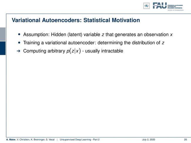
CC BY 4.0 from the 深度学习讲座中 Deep Learning Lecture. CC BY 4.0下的图像。Well, the assumption here is that we have some hidden latent variable z that generates some observation x. Then you can train the variational autoencoder by determining the distribution of z. Then, the problem is that the computation of this distribution p(z|x) is usually intractable. So, we somehow have to approximate our p(z|x) by a tractable distribution. This means that the tractable distribution q then leads to the problem that we have to determine the parameters of q. For example, you can use a Gaussian distribution for this. Then, you can use this to define Kullback-Leibler Divergence between P(z|x) and q(z|x). This is equivalent to maximizing the reconstruction likelihood of the expected value of the logarithm of p(x|z) minus the KL divergence between q(z|x) and p(z). This forces q(z|x) to be similar to the true prior distribution p(z).
好吧,这里的假设是,我们有一些隐藏的潜在变量z生成了一些观测值x。 然后,您可以通过确定z的分布来训练变分自动编码器。 然后,问题在于该分布p( z | x )的计算通常是棘手的。 因此,我们必须以某种易处理的分布来近似逼近我们的p( z | x )。 这意味着可处理的分布q然后导致我们必须确定q的参数的问题。 例如,您可以为此使用高斯分布。 然后,您可以使用它来定义P( z | x )和q( z | x )之间的Kullback-Leibler散度。 这等效于最大化p( x | z )对数的期望值减去q( z | x )和p( z )之间的KL散度的重构可能性。 这迫使q( z | x )类似于真实的先验分布p( z )。
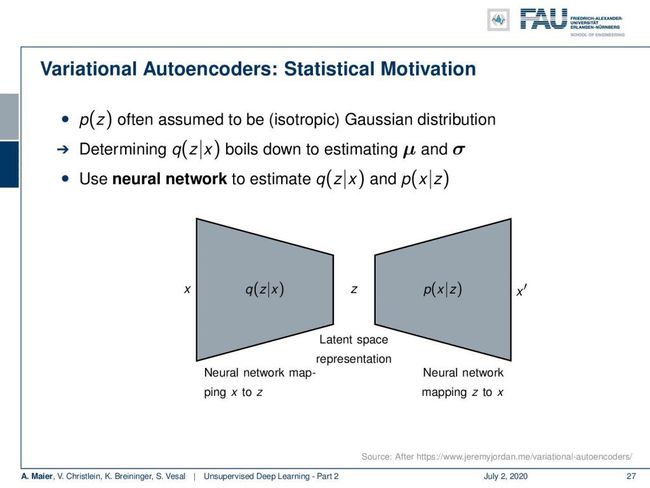
CC BY 4.0 from the 深度学习讲座中 Deep Learning Lecture. CC BY 4.0下的图像。So now, p(z) is often assumed to be the isotropic Gaussian distribution. Determining now q(z|x) boils down to estimating the parameter vectors μ and σ. So, we do this using a neural network. Who might have guessed that? We estimate our q(z|x) and p(x|z). So here, you see the general outline. Again, you see this autoencoder structure and we have this encoder q(z|x) that produces the latent space representation and then our p(x|z) that produces again our output x’. x’ is supposed to be similar to x.
因此,现在通常假定p( z )是各向同性的高斯分布。 现在确定q( z | x )归结为估计参数向量μ和σ 。 因此,我们使用神经网络来做到这一点。 谁会猜到呢? 我们估计q( z | x )和p( x | z )。 因此,在这里,您将看到总体轮廓。 再次,您会看到这种自动编码器结构,并且我们有一个编码器q( z | x )生成潜在空间表示,然后是我们的p( x | z )再次生成我们的输出x '。 x '应该类似于x 。
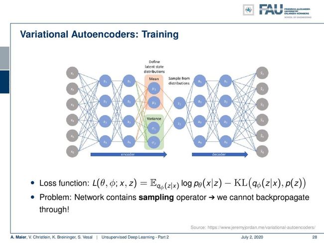
CC BY 4.0 from the 深度学习讲座中 Deep Learning Lecture. CC BY 4.0下的图像。So, let’s look at this in some more detail. You can see that in the encoder branch, we essentially have a classic home feed-forward neural network that reduces the dimensionality. What we do in the following is we introduce one key change. This is indicated here in light red and light green. The key idea here now is that in the specific layer that is indicated by the colors, we change the interpretation of the activations. In those neurons, they’re essentially just feed-forward layers, but we interpret the top two neurons here as means of our latent distribution and the bottom two neurons as variances of the latent distributions. Now, the key problem is that in order to go to the next layer, we have to sample from those distributions in order to get the actual observations and perform the decoding on them. So how can this potentially be done? Well, we have a problem here because we cannot backpropagate through the random sampling process.
因此,让我们更详细地看一下。 您可以看到,在编码器分支中,我们本质上有一个经典的前馈神经网络,它可以降低维数。 下面我们要做的是介绍一个关键的更改。 在此以浅红色和浅绿色指示。 现在的关键思想是,在由颜色指示的特定层中,我们更改激活的解释。 在这些神经元中,它们本质上只是前馈层,但我们在这里将顶部的两个神经元解释为潜在分布的方式,将底部的两个神经元解释为潜在分布的方差。 现在,关键问题是,为了进入下一层,我们必须从这些分布中进行采样,以便获得实际的观测值并对其进行解码。 那么如何才能做到这一点呢? 好吧,我们这里有一个问题,因为我们无法在随机采样过程中反向传播。
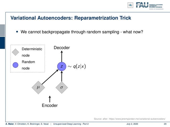
CC BY 4.0 from the 深度学习讲座中 Deep Learning Lecture. CC BY 4.0下的图像。So the idea here is that the encoder produces the means and variances. Then, we produce some z that is a sampling of our function q(z|x). So, this is a random node and the randomness has the problem that we don’t know how to backpropagate for this node. So, the key element that we introduced in the forward-pass here is that we reparameterize z. z is determined deterministically as the μ plus σ times some ε. ε is the random information. It now stems from a random generator that is simply connected to z. For example, you can choose it to be a Gaussian distribution with zero mean and unit variance. So, this then allows us to backpropagate into μ and σ because the random node is here on the right-hand side and we don’t need to backpropagate into the random node. So, by this reparametrization trick, we can even introduce sampling into a network as a layer. So, this is pretty exciting and as you have already guessed. this is also very nice because we can then use this noise in order to generate random samples from this specific distribution. So, we can use the right-hand side of our autoencoder in order to produce new samples. All of this is deterministic in the backpropagation and you can compute your gradients in the same way as we used to. You can apply your backpropagation algorithm as before.
因此,这里的想法是编码器产生均值和方差。 然后,我们生成一些z ,它是函数q( z | x )的采样。 因此,这是一个随机节点,并且随机性具有我们不知道如何向该节点反向传播的问题。 因此,我们在前向传递中引入的关键元素是重新参数化z 。 当μ加σ乘以ε时,确定地确定z 。 ε是随机信息。 现在,它源自简单地连接到z的随机生成器。 例如,您可以将其选择为均值和单位方差为零的高斯分布。 因此,这使我们可以反向传播为μ和σ,因为随机节点在右侧,并且我们不需要反向传播为随机节点。 因此,通过这种重新参数化技巧,我们甚至可以将采样作为一个层引入网络。 因此,这非常令人兴奋,正如您已经猜到的那样。 这也非常好,因为我们可以使用该噪声以便从此特定分布生成随机样本。 因此,我们可以使用自动编码器的右侧来生成新样本。 所有这些在反向传播中都是确定性的,您可以像以前一样计算梯度。 您可以像以前一样应用反向传播算法。
CC BY 4.0 from the 深度学习讲座中 Deep Learning Lecture. CC BY 4.0下的图像。So what effect does this have? Well here, we have some latent space visualizations. If you use only the reconstruction loss, you can see that samples are well separated but there is no smooth transition. Obviously, if you only had the KL divergence then you would not be able to describe the original data. So, you need the combination where you’re simultaneously optimizing with respect to the input distributions and the respective KL divergence. So, this is pretty cool because then we can generate new data by sampling from the distributions in the latent space and then you reconstruct with the decoder the diagonal prior enforces independent latent variables
那么这有什么作用呢? 在这里,我们有一些潜在的空间可视化。 如果仅使用重建损失,则可以看到样本分离得很好,但是没有平滑过渡。 显然,如果仅存在KL散度,则将无法描述原始数据。 因此,您需要组合,同时针对输入分布和各自的KL散度进行优化。 因此,这很酷,因为这样我们就可以通过从潜在空间中的分布中采样来生成新数据,然后使用解码器重构对角先验强制独立的潜在变量
CC BY 4.0 from the 深度学习讲座中 Deep Learning Lecture. CC BY 4.0下的图像。So, we can encode different factors of variation. Here, we have an example where we smoothly vary the degree of smiling and the head pose. You can see that this kind of disentangling actually works.
因此,我们可以编码不同的变异因素。 在这里,我们有一个示例,其中我们平稳地改变了微笑的程度和头部姿势。 您可以看到这种解开确实有效。
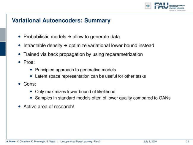
Latent space exploration in variational autoencoders. Image created using gifify. Source: YouTube 变分自动编码器中的潜在空间探索。 使用 gifify创建的 图像 。 资料来源: YouTubeSo, let’s summarize. The variational autoencoder is a probabilistic model that allows you to generate data from an intractable density. We are able to optimize a variational lower bound instead and this is trained by backpropagation using reparametrization.
因此,让我们总结一下。 可变自动编码器是一种概率模型,可让您根据难以处理的密度生成数据。 我们能够优化变分下界,这是通过使用重新参数化的反向传播进行训练的。
CC BY 4.0 from the 深度学习讲座中 Deep Learning Lecture. CC BY 4.0下的图像。The pros are that we have a principled approach to generative modeling. The latent space representation can be very useful for other tasks but the cons are that this only maximizes a lower bound of likelihood. So, the samples in standard models are often of lower quality compared to generative adversarial networks. This is still an active area of research. So, in this video, I gave you a very nice wrap up of autoencoders and the important techniques are, of course, the simple autoencoder, the undercomplete autoencoder, the sparse autoencoder, and the stacked autoencoder. Finally, we’ve been looking into variational autoencoders in order to be able to also generate data and in order to be able to describe probability distributions in our latent variable space.
优点是我们有一种生成建模的原则方法。 潜在空间表示对于其他任务可能非常有用,但是缺点是这只会使可能性的下限最大化。 因此,与生成对抗网络相比,标准模型中的样本通常质量较低。 这仍然是一个活跃的研究领域。 因此,在此视频中,我为您提供了很好的自动编码器包装,而重要的技术当然是简单的自动编码器,欠完善的自动编码器,稀疏的自动编码器和堆叠式自动编码器。 最后,我们一直在研究变分自动编码器,以便能够生成数据并能够描述潜在变量空间中的概率分布。
CC BY 4.0 from the 深度学习讲座中 Deep Learning Lecture. CC BY 4.0下的图像。In the next video, we will see that data generation is a very interesting task and we can essentially do it from unsupervised data. This is why we will look into the generative adversarial networks. You will see that this is a very interesting technique that has led to widespread use in many different applications in order to use the power of deep neural networks to perform data generation. So, I hope you liked this video. We discussed very important points of unsupervised learning and I think these are state-of-the-art techniques that are widely used. So, if you like this video, please stay tuned and looking forward to meeting you in the next one. Thank you very much. Goodbye!
在下一个视频中,我们将看到数据生成是一个非常有趣的任务,并且我们可以从无监督的数据中完成它。 这就是为什么我们将研究生成对抗网络的原因。 您将看到,这是一种非常有趣的技术,已导致在许多不同的应用程序中得到广泛使用,以便利用深度神经网络的强大功能执行数据生成。 所以,我希望你喜欢这个视频。 我们讨论了无监督学习的重要方面,我认为这些是被广泛使用的最新技术。 因此,如果您喜欢此视频,请继续关注,期待与您在下一个视频中见面。 非常感谢你。 再见!
If you liked this post, you can find more essays here, more educational material on Machine Learning here, or have a look at our Deep LearningLecture. I would also appreciate a follow on YouTube, Twitter, Facebook, or LinkedIn in case you want to be informed about more essays, videos, and research in the future. This article is released under the Creative Commons 4.0 Attribution License and can be reprinted and modified if referenced. If you are interested in generating transcripts from video lectures try AutoBlog.
如果你喜欢这篇文章,你可以找到这里更多的文章 ,更多的教育材料,机器学习在这里 ,或看看我们的深入 学习 讲座 。 如果您希望将来了解更多文章,视频和研究信息,也欢迎关注YouTube , Twitter , Facebook或LinkedIn 。 本文是根据知识共享4.0署名许可发布的 ,如果引用,可以重新打印和修改。 如果您对从视频讲座中生成成绩单感兴趣,请尝试使用AutoBlog 。
链接 (Links)
Link — Variational Autoencoders: Link — NIPS 2016 GAN Tutorial of GoodfellowLink — How to train a GAN? Tips and tricks to make GANs work (careful, noteverything is true anymore!) Link - Ever wondered about how to name your GAN?
链接 —可变自动编码器: 链接 — Goodfellow的NIPS 2016 GAN教程链接 —如何训练GAN? 使GAN正常工作的提示和技巧(小心,什么都没了!) 链接 -是否想知道如何命名GAN?
翻译自: https://towardsdatascience.com/unsupervised-learning-part-2-b1c130b8815d
无监督学习 k-means
