机器学习python逻辑回归——多分类(吴恩达课后作业)

一、引入库和数据集

import numpy as np
import scipy.io as io
import matplotlib.pyplot as plt
data=io.loadmat('C:/Users/Administrator/Desktop/新建文件夹/ex3data1.mat')      #type(data)-----dict
data.keys()  #字典data的键有哪些，以列表的形式给出
#dict_keys(['__header__', '__version__', '__globals__', 'X', 'y'])
X=data['X']  #字典data对应键为'X'的值
y=data['y']​
X.shape  #(5000,400) 
y.shape  #(5000, 1)
np.unique(y) 
#array([ 1,  2,  3,  4,  5,  6,  7,  8,  9, 10], dtype=uint8)

数据集data的信息：

二、数据可视化

1.随机打印一个数字

def plot_a_image():
    random_num=np.random.randint(0,5000)  #根据给定的由低到高的范围抽取随机整数
    image=X[random_num,:].reshape(20,20)
    fig,ax=plt.subplots(figsize=(1,1))
    ax.matshow(image.T,cmap='gray_r') #这里为什么要加转置呢？
    '''不加转置的话，可视化的数字是反着的'''
    plt.xticks([]) #去掉刻度，美观
    plt.yticks([])
    plt.show()
    print('这应该是{}'.format(y[random_num]))    

结果如下：

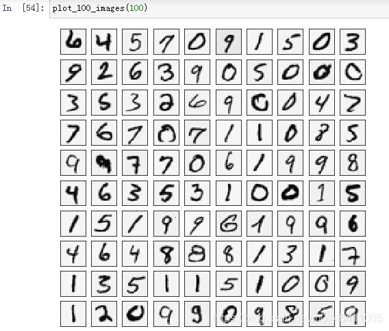
2.随机打印100个数字

def plot_100_images():
    random_sample=np.random.choice(range(0,5000),100)   #range(X.shape[0])
    images=X[random_sample,:]   #(100,10)
    y_images=y.ravel()[random_sample]
    fig,ax_array=plt.subplots(figsize=(8,8),nrows=10,ncols=10,sharex=True,sharey=True)
    for row in range(10):
        for col in range(10):
            ax_array[row,col].matshow((images[row*10+col].reshape(20,20)).T,cmap='gray_r')
    plt.xticks([])
    plt.yticks([])
    plt.show()
    
    fact_number=[]
    for row in range(10):
        for col in range(10):
            fact_number.append(y_images[row*10+col])
    fact_number=np.array(fact_number).reshape(10,10)
    print(fact_number)

三、定义输入变量和标签变量

X=np.insert(X,0,1,axis=1)  #(5000,401)
y=y.ravel()   #(5000,)
theta=np.zeros(X.shape[1])   #(401,)

四、定义代价函数

1.代价函数

def sigmoid(z):
    return 1/(1+np.exp(-z))
def cost(theta,X,y):
    first=y@np.log(sigmoid(X@theta))
    second=(1-y)@np.log(1-sigmoid(X@theta))
    return (first+second)/(-len(X))    

2.正则化后的代价函数

def costReg(theta,X,y,lam=1):
    thetaReg=theta[1:]
    reg=lam/(2*len(X))*np.sum(np.power(thetaReg,2))
    return cost(theta,X,y)+reg

五、梯度函数

1.梯度函数

def gradient(theta,X,y):
    return X.T@sigmoid(X@theta-y)/(-len(X))

2.正则化后的梯度函数

def gradientReg(theta,X,y,lam=1):
    thetaReg=theta[1:]  #第一项没有惩罚因子
    reg=lam/(len(X))*thetaReg
    reg=np.concatenate([np.array([0]),reg])  # np.concatenate()连接
    return gradient(theta,X,y)+reg

六、一对多分类

np.unique(y)
#array([ 1,  2,  3,  4,  5,  6,  7,  8,  9, 10], dtype=uint8)

所以建立十个逻辑分类器，每个逻辑分类器是二分类。

import scipy.optimize as opt
def one_vs_all(X,y,K):  #K是指要分成K个类
    all_theta=np.zeros((K,X.shape[1])) # K个分类器的最终权重
    for i in range(1,K+1): #因为y的取值为1，，，，10
        theta=np.zeros(X.shape[1])  #第i个分类器的权重
        y_i=np.array([1 if label==i else 0 for label in y])
        #将y的值划分为二分类：0和1
        res=opt.minimize(fun=costReg,x0=theta,args=(X,y_i,1),method='TNC',jac=gradientReg,options={'disp':True})
        #Whether to print the result rather than returning it
        all_theta[i-1,:]=res.x
    return all_theta
all_theta=one_vs_all(X,y,10)

七、预测

all_theta.shape  #(10,401)
def predict_all(theta,X):
    h=sigmoid(X@theta.T)
    y_argmax=np.argmax(h,axis=1)
    y_pred=y_argmax+1
    return y_pred

y_pred=predict_all(all_theta,X)
y_pred #array([10, 10, 10, ...,  9,  9,  7], dtype=int64)
y  #array([10, 10, 10, ...,  9,  9,  9], dtype=uint8)
accuracy=np.mean(y_pred==y)
accuracy   #0.9446