技巧 | 使用基础绘图系统绘制「森林图」

森林图可以很直观地表达数学模型的结果，尤其是在对比多种情境的结果时。

R语言中有一些专门绘制森林图的工具包，不过小编目前还没仔细研究过。实际上，通过基础绘图系统的一些简单函数的组合使用就能绘制森林图。

首先生成用于绘图的模型结果：

## 全样本模型
data = mtcars
model = lm(mpg ~ qsec, data)
coeff = summary(model)$coefficients[2, 1] 
se = summary(model)$coefficients[2, 2] 

## 子样本模型
for(i in 3:5) {
  model.1 <- lm(mpg ~ qsec, data,
                subset = gear == i)
  coeff[i-1] = summary(model.1)$coefficients[2, 1] 
  se[i-1] = summary(model.1)$coefficients[2, 2] 
}

## 结果整理
library(tidyverse)
result <- tibble(
  coeff = coeff,
  se = se,
  lower = coeff - 1.96*se,
  upper = coeff + 1.96*se
)

result
## # A tibble: 4 x 4
##   coeff    se   lower upper
##        
## 1 1.41  0.559  0.316   2.51
## 2 1.22  0.604  0.0393  2.41
## 3 0.853 0.998 -1.10    2.81
## 4 5.77  0.685  4.43    7.11

❝

• 上述结果中，coeff为模型系数，lower和upper为95%置信区间的下限和上限。

❞

下面的代码提供了绘制森林图的基本思路：

plot(1, xlim = c(0,4), ylim = c(0,4),
     type = "n", ann = F)
abline(h = 0:4, col = "grey")
points(rep(3,4), (0:3)+0.5, 
       pch = 21, bg = "black")
set.seed(999)
segments(3-runif(4), (3:0)+0.5,
         3+runif(4), (3:0)+0.5)

❝

• 使用plot()函数生成绘图页面，之后的函数如abline()、points()等都是低级函数；

• 在plot()函数中，根据需要设置横、纵坐标的范围；type = n表示隐藏图形，只输出空白页面；

• abline()函数用来根据需要绘制格网（图中为水平线）；

• points()函数绘制中心点；

• segments()函数绘制置信区间的连线。

❞

在上述框架内，坐标范围的设置与绘图数据无关，因此需要建立二者的映射关系。

例如，使用图形中横坐标在[2,4]之间的区域来绘制森林图，这样就需要把原始数据转换到该区间内。

min(result)
## [1] -1.102983

max(result)
## [1] 7.112582

根据绘图数据result的实际范围，需要将区间[-2,7.5]（「数据区间」）映射到区间[2,4]（「图形区间」）上去。这个过程实际就是已知两点去求直线方程，可以通过定义如下函数f()来实现：

f = function(x) {
  r1 = c(-2,7.5)
  r2 = c(2,4) 
  b = (lm(r2 ~ r1))$coefficients
  return(x*b[2] + b[1])
}

result2 = f(result)
result2
##      coeff       se    lower    upper
## 1 2.718342 2.538781 2.487594 2.949090
## 2 2.678550 2.548206 2.429329 2.927770
## 3 2.600697 2.631181 2.188846 3.012549
## 4 3.635697 2.565308 3.352956 3.918438

❝

• result2就是转换后的数据，所有数值均在[2,4]之间。

❞

将前面绘图代码中points()和segments()函数中的相关参数值改成result2中对应的变量：

plot(1, xlim = c(0,4), ylim = c(0,4),
     type = "n", ann = F)
abline(h = 0:4, col = "grey")
## result2$coeff
points(result2$coeff, (3:0)+0.5, 
       pch = 21, bg = "black")
## result2$lower和result2$upper
segments(result2$lower, (3:0)+0.5,
         result2$upper, (3:0)+0.5)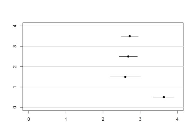

上述图形虽然已经能表达绘图数据的结果了，但它的坐标轴刻度与绘图数据是不对应的。

绘图数据所需要的刻度与图形实际的刻度之间也可以通过前面定义的f()函数进行转换：

xx = seq(-2, 8, 2)
xx0 = f(xx)

在plot()函数中添加axes = F语句隐去图形的实际刻度，再使用低级函数axis()添加新的坐标刻度。

par(plt = c(0.05,0.95,0.2,0.8))
plot(1, xlim = c(0,4), ylim = c(0,4),
     type = "n", ann = F, axes = F)
abline(h = 0:4, col = "grey")
points(result2$coeff, (3:0)+0.5, 
       pch = 21, bg = "black")
segments(result2$lower, (3:0)+0.5,
         result2$upper, (3:0)+0.5)
## 添加坐标刻度
axis(1, at = xx0, labels = xx)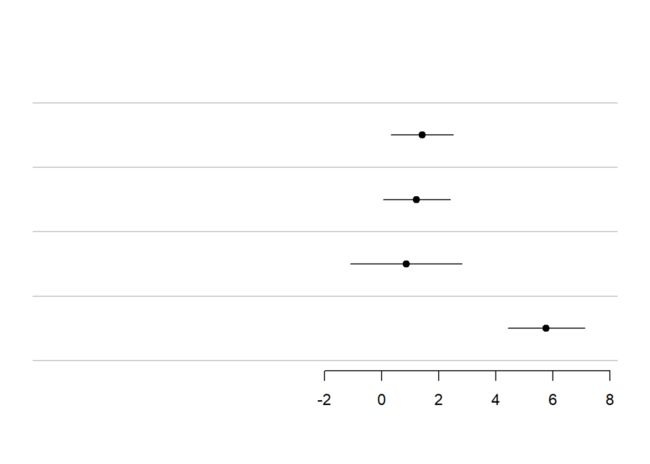

至此，森林图已经成型了。在图形左侧还可以根据需要添加相关标注，如添加如下文本。

result3 = round(result, 2)
text = paste0(result3$coeff, "(", result3$lower,
              "-", result3$upper, ")")
text
## [1] "1.41(0.32-2.51)" "1.22(0.04-2.41)" "0.85(-1.1-2.81)" "5.77(4.43-7.11)"

使用低级函数text()将文本添加到图形对应位置上：

par(plt = c(0.05,0.95,0.2,0.8))
plot(1, xlim = c(0,4), ylim = c(0,4),
     type = "n", ann = F, axes = F)
abline(h = 0:4, col = "grey")
points(result2$coeff, (3:0)+0.5, 
       pch = 21, bg = "black")
segments(result2$lower, (3:0)+0.5,
         result2$upper, (3:0)+0.5)
axis(1, at = xx0, labels = xx)
## 添加文本
text(rep(1,4), (3:0)+0.5, text, family = "mono")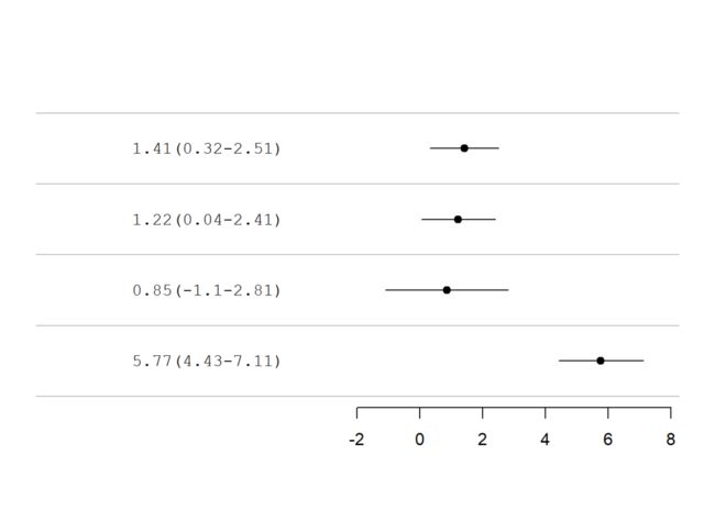

还可以根据需要进行其他修饰，这里再次使用低级函数abline()添加格网（竖直线）：

par(plt = c(0.05,0.95,0.2,0.8))
plot(1, type = "n", ann = F, xlim = c(0,4), ylim = c(0,4),
     axes = F)
abline(h = 0:4, col = "grey")
points(result2$coeff, (3:0)+0.5, 
       pch = 21, bg = "black")
segments(result2$lower, (3:0)+0.5,
         result2$upper, (3:0)+0.5)
axis(1, at = xx0, labels = xx)
text(rep(1,4), (3:0)+0.5, text, family = "mono") 
## 添加格网
abline(v = xx0, col = "grey", lty = 2)

❝

• segments()函数也可以用来添加格网。

❞

以上就是仅使用基础绘图系统的函数绘制一个简单森林图的过程，更复杂的情况则可以通过各种细节进行调整去实现。