18_3Reinforcement Learning_LunarLander_SpaceInvader
cp18_Reinforcement Learning for Markov Decision Making in Env_Bellman_Q-learning_Q-Value Iteration : https://blog.csdn.net/Linli522362242/article/details/117889535
Exercises
1. How would you define Reinforcement Learning? How is it different from regular supervised or unsupervised learning?
Reinforcement Learning is an area of Machine Learning aimed at creating agents
capable of taking actions in an environment in a way that maximizes rewards
over time. There are many differences between RL and regular supervised and
unsupervised learning. Here are a few:
- • In supervised and unsupervised learning, the goal is generally to find patterns in the data and use them to make predictions.
In Reinforcement Learning, the goal is to find a good policy.
- • Unlike in supervised learning, the agent is not explicitly given the “right” answer. It must learn by trial and error.
- • Unlike in unsupervised learning, there is a form of supervision, through rewards. We do not tell the agent how to perform the task, but we do tell it when it is making progress or when it is failing.
- • A Reinforcement Learning agent needs to find the right balance between exploring the environment, looking for new ways of getting rewards, and exploiting sources of rewards that it already knows.
In contrast, supervised and unsupervised learning systems generally don’t need to worry about exploration; they just feed on the training data they are given.
- • In supervised and unsupervised learning, training instances are typically independent (in fact, they are generally shuffled).
In Reinforcement Learning, consecutive observations are generally not independent. An agent may remain in the same region of the environment for a while before it moves on, so consecutive observations will be very correlated.
In some cases a replay memory (buffer) is used to ensure that the training algorithm gets fairly independent observations.
2. Can you think of three possible applications of RL that were not mentioned in this chapter? For each of them, what is the environment? What is the agent? What are some possible actions? What are the rewards?
- Music personalization音乐个性化
The environment is a user’s personalized web radio个性化网络广播.
The agent is the software deciding what song to play next for that user. Its possible actions are to play any song in the catalog (it must try to choose a song the user will enjoy) or to play an advertisement (it must try to choose an ad that the user will be interested in). It gets a small reward every time the user listens to a song, a larger reward every time the user listens to an ad, a negative reward when the user skips a song or an ad, and a very negative reward if the user leaves.
- Marketing
The environment is your company’s marketing department.
The agent is the software that defines which customers a mailing campaign活动 should be sent to, given their profile and purchase history (for each customer it has two possible actions: send or don’t send). It gets a negative reward for the cost of the mailing campaign, and a positive reward for estimated revenue generated from this campaign.
- Product delivery
Let the agent control a fleet队 of delivery trucks, deciding what they should pick up at the depots仓库, where they should go, what they should drop off, and so on. It will get positive rewards for each product delivered on time, and negative rewards for late deliveries.
3. What is the discount factor? Can the optimal policy change if you modify the discount factor?
When estimating the value of an action, Reinforcement Learning algorithms typically sum all the rewards that this action led to, giving more weight to immediate rewards and less weight to later rewards (considering that an action has more influence on the near future than on the distant future). To model this, a discount factor is typically applied at each time step.
For example, with a discount factor of 0.9, a reward of 100 that is received two time steps later is counted as only 0.92 × 100 = 81 when you are estimating the value of the action. You can think of the discount factor as a measure of how much the future is valued relative to the present: if it is very close to 1, then the future is valued almost as much as the present; if it is close to 0, then only immediate rewards matter. Of course, this impacts the optimal policy tremendously: if you value the future, you may be willing to put up with a lot of immediate pain for the prospect of eventual rewards, while if you don’t value the future, you will just grab any immediate reward you can find, never investing in the future.
4. How do you measure the performance of a Reinforcement Learning agent?
To measure the performance of a Reinforcement Learning agent, you can simply sum up the rewards it gets.
In a simulated environment, you can run many episodes and look at the total rewards it gets on average (and possibly look at the min, max, standard deviation, and so on).
5. What is the credit assignment problem? When does it occur? How can you alleviate it?
The credit assignment problem is the fact that when a Reinforcement Learning agent receives a reward, it has no direct way of knowing which of its previous actions contributed to this reward. It typically occurs when there is a large delay between an action and the resulting reward (e.g., during a game of Atari’s Pong, there may be a few dozen time steps between the moment the agent hits the ball and the moment it wins the point). One way to alleviate it is to provide the agent with shorter-term rewards, when possible. This usually requires prior knowledge about the task. For example, if we want to build an agent that will learn to play chess, instead of giving it a reward only when it wins the game, we could give it a reward every time it captures one of the opponent’s pieces.
6. What is the point of using a replay buffer?
An agent can often remain in the same region of its environment for a while, so all of its experiences will be very similar for that period of time. This can introduce some bias in the learning algorithm. It may tune its policy for this region of the environment, but it will not perform well as soon as it moves out of this region. To solve this problem, you can use a replay memory; instead of using only the most immediate experiences for learning, the agent will learn based on a buffer of its past experiences, recent and not so recent (perhaps this is why we dream at night: to replay our experiences of the day and better learn from them?).
7. What is an off-policy RL algorithm?
An off-policy RL algorithm learns the value of the optimal policy (i.e., the sum of discounted rewards that can be expected for each state if the agent acts optimally) while the agent follows a different policy. Q-Learning is a good example of such an algorithm.
In contrast, an on-policy algorithm learns the value of the policy that the agent actually executes, including both exploration and exploitation.
8. Use policy gradients to solve OpenAI Gym’s LunarLander-v2 environment. You will need to install the Box2D dependencies (python3 -m pip install -U gym[box2d]).
!python3 -m pip install -U gym[box2d] Let's start by creating a LunarLander-v2 environment:
import gym

env = gym.make( "LunarLander-v2" )
The inputs are 8-dimensional:
env.observation_space![]()
env.seed(42)
obs = env.reset()
obs![]()
From the source code
(https://github.com/openai/gym/blob/master/gym/envs/box2d/lunar_lander.py), we can see that these each 8D observation (x, y, h, v, a, w, l, r) correspond to:
- x,y:
the coordinates of the spaceship. It starts at a random location near (0, 1.4) and must land near the target at (0, 0). - h,v:
the horizontal and vertical speed of the spaceship. It starts with a small random speed. - a,w:
the spaceship's angle and angular velocity. - l,r:
whether the left or right leg touches the ground (1.0) or not (0.0).
The action space is discrete, with 4 possible actions:
env.action_space![]()
Looking at the LunarLander-v2's description,(https://gym.openai.com/envs/LunarLander-v2/) these actions are:
- do nothing
- fire left orientation engine
- fire main engine
- fire right orientation engine
Let's create a simple policy network with 4 output neurons (one per possible action):
from tensorflow import keras
import numpy as np
import tensorflow as tf

keras.backend.clear_session()
np.random.seed(42)
tf.random.set_seed(42)

n_inputs = env.observation_space.shape[0] # (8,)
n_outputs = env.action_space.n            # 4

model = keras.models.Sequential([
            keras.layers.Dense( 32, activation="relu", input_shape=[n_inputs] ),
            keras.layers.Dense( 32, activation="relu" ),
            keras.layers.Dense( n_outputs, activation="softmax" ),
        ])
Note that we're using the softmax activation function in the output layer, instead of the sigmoid activation function like we did for the CartPole-v1 environment. This is because we only had two possible actions for the CartPole-v1 environment, so a binary classification model worked fine. However, since we now how more than two possible actions, we need a multiclass classification model (env.action_space.n ==4).
Next, let's reuse the play_one_step() and play_multiple_episodes() functions we defined for the CartPole-v1 Policy Gradient code above, but we'll just tweak the play_one_step() function to account for the fact that the model is now a multiclass classification model rather than a binary classification model. We'll also tweak the play_multiple_episodes() function to call our tweaked play_one_step() function rather than the original one, and we add a big penalty if the spaceship does not land (or crash) before a maximum number of steps.
def lander_play_one_step( env, obs, model, loss_fn ):
  with tf.GradientTape() as tape:
    probas = model( obs[np.newaxis] ) # obs[np.newaxis] ==> (batch_size, observation)
    logits = tf.math.log( probas + keras.backend.epsilon() )
    # num_samples : Number of independent samples to draw for each row slice.
    # tf.random.categorical : The drawn samples of shape [batch_size, num_samples].
    action = tf.random.categorical( logits, num_samples=1 ) # select an action index for each sample
    loss = tf.reduce_mean( loss_fn(action, probas) )
  grads = tape.gradient( loss, model.trainable_variables )
  obs, reward, done, info = env.step( action[0,0].numpy() )
  return obs, reward, done, grads

def lander_play_multiple_episodes( env, n_episodes, n_max_steps, model, loss_fn ):
  all_rewards = []
  all_grads = []

  for episode in range( n_episodes ):
    current_rewards = []
    current_grads = []
    obs = env.reset()

    for step in range( n_max_steps ):
      obs, reward, done, grads = lander_play_one_step( env, obs, model, loss_fn )
      current_rewards.append( reward )
      current_grads.append( grads )
      if done:
        break

    all_rewards.append( current_rewards )
    all_grads.append( current_grads )

  return all_rewards, all_grads
We'll keep exactly the same discount_rewards() and discount_and_normalize_rewards() functions as earlier:
# https://blog.csdn.net/Linli522362242/article/details/117673730
def discount_rewards( rewards, discount_rate ):
  discounted = np.array( rewards )
  # from back to front that to avoid use a recursion
  for step in range( len(rewards)-2, -1, -1 ): # except last_reward(use itself): len(rewards)-1
    discounted[step] += discounted[step+1] * discount_rate
  return discounted

# To normalize all discounted rewards across all episodes
def discount_and_normalize_rewards( all_rewards, discount_rate ):
  all_discounted_rewards = [ discount_rewards(rewards, discount_rate)
                             for rewards in all_rewards
                           ]
  flat_rewards = np.concatenate( all_discounted_rewards ) # []+...[]=>[]
  reward_mean = flat_rewards.mean()
  reward_std = flat_rewards.std()

  return[ (discounted_rewards - reward_mean)/reward_std
          for discounted_rewards in all_discounted_rewards
        ]
Now let's define some hyperparameters:
n_iterations = 200
n_episodes_per_update = 16
n_max_steps = 1000
discount_rate = 0.99
Again, since the model is a multiclass classification model, we must use the categorical cross-entropy rather than the binary cross-entropy. Moreover, since the lander_play_one_step() function sets the targets as class indices(action = tf.random.categorical( logits, num_samples=1 )) rather than class probabilities, we must use the sparse_categorical_crossentropy() loss function:
optimizer = keras.optimizers.Nadam( learning_rate=0.005 )
loss_fn = keras.losses.sparse_categorical_crossentropy
We're ready to train the model. Let's go!
env.seed(42)

mean_rewards = []

for iteration in range( n_iterations ):
  all_rewards, all_grads = lander_play_multiple_episodes( env,
                                                          n_episodes_per_update,
                                                          n_max_steps,
                                                          model,
                                                          loss_fn
                                                        )
  mean_reward = sum( map(sum, all_rewards) ) / n_episodes_per_update
  print( "\rIteration: {}/{}, mean reward: {:.1f} ".format( iteration+1,
                                                            n_iterations,
                                                            mean_reward
                                                          ),
        end = ""
       )
  mean_rewards.append( mean_reward )

  all_final_rewards = discount_and_normalize_rewards( all_rewards,
                                                      discount_rate
                                                    )

  all_mean_grads = []
  for var_index in range( len(model.trainable_variables) ):
    mean_grads = tf.reduce_mean(
        [ final_reward * all_grads[episode_index][step][var_index]
          for episode_index, final_rewards in enumerate( all_final_rewards )
            for step, final_reward in enumerate( final_rewards )
        ],
        axis=0
    )
    all_mean_grads.append( mean_grads )

optimizer.apply_gradients( zip( all_mean_grads, model.trainable_variables ) )![]()
Let's look at the learning curve:
import matplotlib.pyplot as plt

plt.plot( mean_rewards )
plt.xlabel( "Episode" )
plt.ylabel( "Mean reward" )
plt.grid()

plt.show()
Now let's look at the result!
def lander_render_policy_net( model, n_max_stepss=500, seed=42 ):
  frames = []
  env = gym.make( "LunarLander-v2" )

  env.seed(seed)
  tf.random.set_seed(seed)
  np.random.seed(seed)

  obs = env.reset()

  for step in range( n_max_steps ):
    frames.append( env.render(mode="rgb_array") )
    probas = model( obs[np.newaxis] )
    logits = tf.math.log( probas + keras.backend.epsilon() )
    action = tf.random.categorical( logits, num_samples=1 )
    obs, reward, done, info = env.step( action[0,0].numpy() )
    if done:
      break
  env.close()
  return frames
from IPython import display as ipythondisplay
from pyvirtualdisplay import Display
import matplotlib.animation as animation
import matplotlib as mpl
mpl.rc('animation', html='jshtml')
def update_scene( num, frames, patch ):
patch.set_data( frames[num] )
return patch,
def plot_animation( frames, repeat=False, interval=40 ):
fig = plt.figure()
patch = plt.imshow( frames[0] ) # img
plt.axis( 'off' )
anim = animation.FuncAnimation(
fig, # figure
func=update_scene, # The function to call at each frame.
fargs=(frames, patch), # Additional arguments to pass to each call to func.
frames = len(frames), # iterable, int, generator function, or None, optional : Source of data to pass func and each frame of the animation
repeat=repeat,
interval=interval
)
plt.close()
return anim
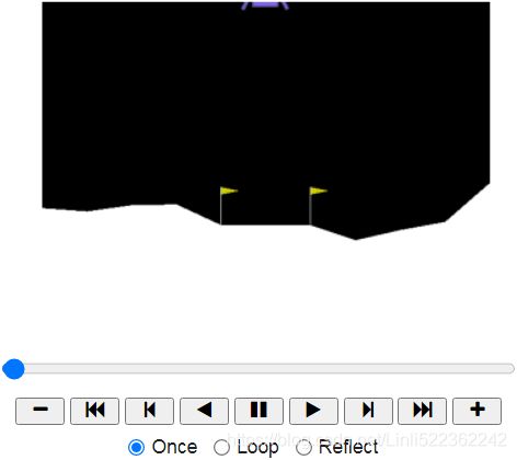
frames = lander_render_policy_net( model, seed=42 )
plot_animation( frames )That's pretty good. You can try training it for longer and/or tweaking the hyperparameters to see if you can get it to go over 200.
import PIL
import os

image_path = os.path.join("/content/drive/MyDrive/Colab Notebooks/hand_on_ml", "LunarLander.gif")
frame_images = [ PIL.Image.fromarray(frame) for frame in frames ]
frame_images[0].save( image_path, format='GIF',
                      append_images=frame_images[1:],
                      save_all=True,
                      duration=30,
                      loop=0
                     )
9. Use TF-Agents to train an agent that can achieve a superhuman level at SpaceInvaders-v4 using any of the available algorithms.
Please follow the steps in the Using TF-Agents to Beat Breakout(The TF-Agents Library https://blog.csdn.net/Linli522362242/article/details/119053283) section above, replacing "Breakout-v4" with "SpaceInvaders-v4". There will be a few things to tweak, however. For example, the Space Invaders game does not require the user to press FIRE to begin the game. Instead, the player's laser cannon[ˈkænən]机关炮 blinks for a few seconds then the game starts automatically. For better performance, you may want to skip this blinking phase (which lasts about 40 steps) at the beginning of each episode and after each life lost. Indeed, it's impossible to do anything at all during this phase, and nothing moves. One way to do this is to use the following custom environment wrapper, instead of the AtariPreprocessingWithAutoFire wrapper: (in colab)
# step 1.
!python3 -m pip install -U 'gym[atari]'
!python3 -m pip install -U tf-agents
!wget http://www.atarimania.com/roms/Roms.rar
!mkdir /content/ROM/
!unrar e /content/Roms.rar /content/ROM/
!python -m atari_py.import_roms /content/ROM/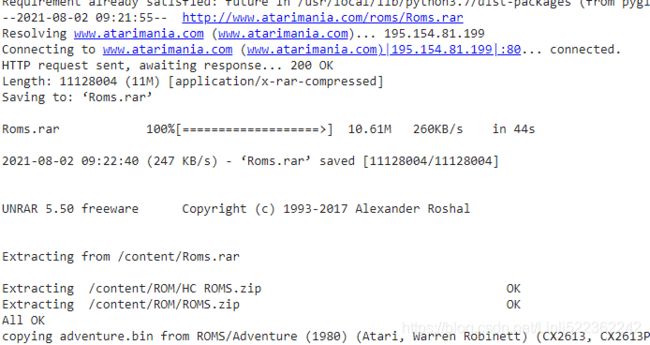
# step 2. Environments
from tf_agents.environments import suite_gym

env = suite_gym.load('SpaceInvaders-v4')
env![]()
This is just a wrapper around an OpenAI Gym environment, which you can access through the gym attribute:
env.gym![]()
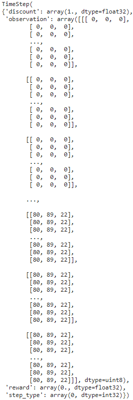
TF-Agents environments are very similar to OpenAI Gym environments, but there are a few differences. First, the reset() method does not return an observation; instead it returns a TimeStep object that wraps the observation, as well as some extra information:
env.seed(42)
env.reset()
The observations are quite large, so we will downsample them
 ==env.step(1)==>
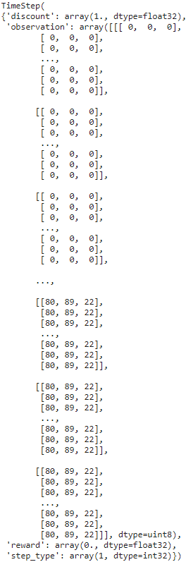
env.step(1)The reward and observation attributes are self-explanatory, and they are the same as for OpenAI Gym (except the reward is represented as a NumPy array). The step_type attribute is equal to
- 0 for the first time step in the episode,
- 1 for intermediate time steps, and
- 2 for the final time step.
You can call the time step’s is_last() method to check whether it is the final one or not. Lastly, the discount attribute indicates the discount factor to use at this time step. In this example it is equal to 1, so there will be no discount at all. You can define the discount factor by setting the discount parameter when loading the environment.
img = env.render( mode = "rgb_array" )
import matplotlib.pyplot as plt
plt.figure( figsize=(6,8) )
plt.imshow( img )
plt.axis( 'off' )
plt.show()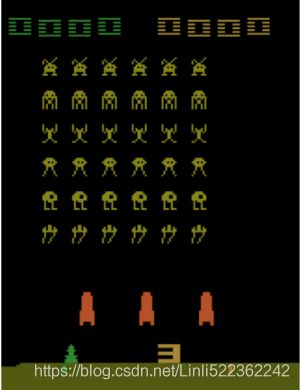 ==>env.current_time_step()
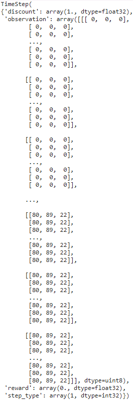
env.current_time_step()Environment Specifications
Specs can be instances of a specification规范 class, nested lists, or dictionaries of specs. If the specification is nested, then the specified object must match the specification’s nested structure. For example, if the observation spec is {"sensors": ArraySpec(shape=[2]), "camera": ArraySpec(shape=[100, 100])}, then a valid observation would be {"sensors": np.array([1.5, 3.5]), "camera": np.array(...)}. The tf.nest package provides tools to handle such nested structures (a.k.a. nests).
Conveniently, a TF-Agents environment provides the specifications of the observations, actions, and time steps, including their shapes, data types, and names, as well as their minimum and maximum values:
env.observation_spec()![]()
Observations vary depending on the environment. In this case it is an RGB image represented as a 3D NumPy array of shape [width, height, channels] (with 3 channels: Red, Green and Blue).
env.action_spec()![]()
env.time_step_spec()
As you can see, the observations are simply screenshots of the SpaceInvaders screen, represented as NumPy arrays of shape [210, 160, 3]. To render an environment, you can call env.render(mode="human"), and if you want to get back the image in the form of a NumPy array, just call env.render(mode="rgb_array") (unlike in OpenAI Gym, this is the default mode).
There are 6 actions available. Gym’s SpaceInvaders environments have an extra method that you can call to know what each action corresponds to:
env.gym.get_action_meanings()![]()
The observations are quite large, so we will downsample them and also convert them to grayscale. This will speed up training and use less RAM. For this, we can use an environment wrapper.
To create a wrapped environment, you must create a wrapper, passing the wrapped environment to the constructor. That’s all! For example, the following code will wrap our environment in an ActionRepeat wrapper so that every action is repeated 4 times:
from tf_agents.environments.wrappers import ActionRepeat

repeating_env = ActionRepeat( env, times=4 )
repeating_env![]()
You can use env.unwrapped to get the original class. The original class takes as long as you want to step, and it will not fail after 200 steps:
repeating_env.unwrapped![]()
OpenAI Gym has some environment wrappers of its own in the gym.wrappers package. They are meant to wrap Gym environments, though, not TF-Agents environments, so to use them you must
- first wrap the Gym environment with a Gym wrapper,
- then wrap the resulting environment with a TF-Agents wrapper.
The suite_gym.wrap_env() function will do this for you, provided you give it a Gym environment and a list of Gym wrappers and/or a list of TF-Agents wrappers.
Alternatively, the suite_gym.load() function will both create the Gym environment and wrap it for you, if you give it some wrappers. Each wrapper will be created without any arguments, so if you want to set some arguments, you must pass a lambda.
For example, the following code creates a SpaceInvaders environment that will run for a maximum of 10,000 steps during each episode, and each action will be repeated 4 times:
from functools import partial
from gym.wrappers import TimeLimit

limited_repeating_env = suite_gym.load(
    "SpaceInvaders-v4",
    gym_env_wrappers = [ partial( TimeLimit, max_episode_steps=10000) ],
    env_wrappers = [ partial( ActionRepeat, times=4) ],
)
For example, the Space Invaders game does not require the user to press FIRE to begin the game. Instead, the player's laser cannon blinks for a few seconds then the game starts automatically. For better performance, you may want to skip this blinking phase (which lasts about 40 steps) at the beginning of each episode and after each life lost. Indeed, it's impossible to do anything at all during this phase, and nothing moves. One way to do this is to use the following custom environment wrapper, instead of the AtariPreprocessingWithAutoFire wrapper:
# step 2_2. Environments
from tf_agents.environments import suite_atari
from tf_agents.environments.atari_preprocessing import AtariPreprocessing
from tf_agents.environments.atari_wrappers import FrameStack4

max_episode_steps = 27000 # == 108k ALE frames since 1 step = 4 frames
environment_name = "SpaceInvaders-v4"

# https://github.com/tensorflow/agents/blob/master/tf_agents/environments/atari_preprocessing.py
class AtariPreprocessingWithSkipStart( AtariPreprocessing ):
  def skip_frames( self, num_skip ):
    for _ in range( num_skip ):
      super().step(0) # NOOP for num_skip steps

  def reset( self, **kwargs ):
    obs = super().reset( **kwargs )
    self.skip_frames( 40 )
    return obs

  def step( self, action ):
    lives_before_action = self.ale.lives()
    obs, rewards, done, info = super().step(action)

    if self.ale.lives() < lives_before_action and not done:
      self.skip_frames(40)

    return obs, rewards, done, info

# https://github.com/tensorflow/agents/blob/master/tf_agents/environments/suite_atari.py
env = suite_atari.load( environment_name,
                        max_episode_steps = max_episode_steps,
                        gym_env_wrappers = [ AtariPreprocessingWithSkipStart,
                                             FrameStack4]
                      )
Play a few steps just to see what happens:
env.seed(42)
env.reset()

for _ in range(4):
  time_step = env.step(3)
The agent only gets to see every n frames of the game (by default n = 4) OR 4 frames per step
env.current_time_step().observation.shape![]()
import numpy as np

def plot_observation( obs ):
    obs = obs.astype( np.float32 )
    img = obs[..., :3]
    img = np.clip( img/150, 0, 1) # clip(a, a_min, a_max, out=None)

    plt.imshow( img )
    plt.axis('off')

plt.figure( figsize=(6,6) )
plot_observation( time_step.observation )

plt.show()
Lastly, we can wrap the environment inside a TFPyEnvironment ( Convert the Python environment to a TF environment ):
from tf_agents.environments.tf_py_environment import TFPyEnvironment

tf_env = TFPyEnvironment( env )
# step 3. Networks
from tf_agents.networks.q_network import QNetwork
from tensorflow import keras
import tensorflow as tf

preprocessing_layer = keras.layers.Lambda(
                                    lambda obs: tf.cast( obs, np.float32)/255. )
conv_layer_params = [ (32, (8,8), 4), # 32, 8 × 8 filter, strides = 4
                      (64, (4,4), 2),
                      (64, (3,3), 1)
                    ]
fc_layer_params = [512] # a dense layer with 512 units

q_net = QNetwork( tf_env.observation_spec(),
                  tf_env.action_spec(),
                  preprocessing_layers = preprocessing_layer,
                  conv_layer_params = conv_layer_params,
                  fc_layer_params = fc_layer_params
                )
# step 4. Agent
epsilon_greedy: probability of choosing a random action in the default epsilon-greedy collect policy (used only if a wrapper is not provided to the collect_policy method). Only one of epsilon_greedy and boltzmann_temperature should be provided
from tf_agents.agents.dqn.dqn_agent import DqnAgent

train_step = tf.Variable(0)
update_period = 4                   # run a training step every 4 collect steps

# https://blog.csdn.net/Linli522362242/article/details/106982127
# https://keras.io/api/optimizers/rmsprop/
optimizer = keras.optimizers.RMSprop( learning_rate=2.5e-4,
                                      rho = 0.95, # Discounting factor for the history/coming gradient. Defaults to 0.9.
                                      momentum = 0.0,
                                      epsilon = 0.00001,
                                      centered = True # Boolean. If True, gradients are normalized by the estimated variance of the gradient;
                                    )
epsilon_fn = keras.optimizers.schedules.PolynomialDecay(
                                                        initial_learning_rate = 1.0, # initial e
                                                        decay_steps = 250000//update_period, # <=> 1,000,000 ALE frames
                                                        end_learning_rate = 0.01    # final e
                                                       )

# https://github.com/tensorflow/agents/blob/master/tf_agents/agents/dqn/dqn_agent.py
agent = DqnAgent( tf_env.time_step_spec(),
                  tf_env.action_spec(),
                  q_network = q_net,
                  optimizer = optimizer,
                  target_update_period = 2000, # ==> 32,000 ALE frames since 1 step = 4 frames, train the agent every 4 steps
                  td_errors_loss_fn = keras.losses.Huber( reduction="none" ),
                  gamma = 0.99,                # discount factor
                  train_step_counter = train_step,
                  epsilon_greedy = lambda: epsilon_fn( train_step )
                )
agent.initialize()
# step 5. Creating the Replay Buffer and the Corresponding Observer
data_spec # A TensorSpec or a list/tuple/nest of TensorSpecs describing a single item that can be stored in this buffer.
The specification of the data that will be saved in the replay buffer. The DQN agent knowns what the collected data will look like, and it makes the data spec available via its collect_data_spec attribute, so that’s what we give the replay buffer.
from tf_agents.replay_buffers import tf_uniform_replay_buffer

replay_buffer = tf_uniform_replay_buffer.TFUniformReplayBuffer(
                                            data_spec = agent.collect_data_spec,
                                            batch_size = tf_env.batch_size,
                                            max_length = 100000 # # reduce if OOM error
                )
replay_buffer_observer = replay_buffer.add_batch
Now we can create the observer that will write the trajectories to the replay buffer. An observer is just a function (or a callable object) that takes a trajectory argument, so we
can directly use the add_method() method (bound to the replay_buffer object) as our observer : replay_buffer_observer = replay_buffer.add_batch
# step 6. Creating Training Metrics
TF-Agents implements several RL metrics in the tf_agents.metrics package, some purely in Python and some based on TensorFlow. Let’s create a few of them in order to count the number of episodes, the number of steps taken, and most importantly the average return per episode and the average episode length:
from tf_agents.metrics import tf_metrics

train_metrics = [
                  tf_metrics.NumberOfEpisodes(),           # count the number of episodes
                  tf_metrics.EnvironmentSteps(),           # the number of steps taken
                  tf_metrics.AverageReturnMetric(),        # the average return per episode
                  tf_metrics.AverageEpisodeLengthMetric(), # the average episode length
                ]
Discounting the rewards makes sense for training or to implement a policy, as it makes it possible to balance the importance of immediate rewards with future rewards. However, once an episode is over, we can evaluate how good it was overalls by summing the undiscounted rewards. For this reason, the AverageReturnMetric computes the sum of undiscounted rewards for each episode, and it keeps track of the streaming mean of these sums over all the episodes it encounters.
Alternatively, you can log all metrics by calling log_metrics(train_metrics) (this function is located in the tf_agents.eval.metric_utils package):
from tf_agents.eval.metric_utils import log_metrics
import logging

logging.getLogger().setLevel( logging.INFO )
log_metrics( train_metrics ) 
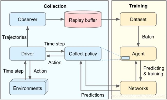
# step 7. Driver
from tf_agents.drivers.dynamic_step_driver import DynamicStepDriver

collect_driver = DynamicStepDriver(
                                    tf_env, # tf_env = TFPyEnvironment( env ) # env = suite_atari.load(...)
                                    agent.collect_policy,     # epsilon_greedy
                                    observers = [replay_buffer_observer] + train_metrics,
                                    num_steps = update_period # collect 4 steps for each training iteration
                                  )
We could now run it by calling its run() method, but it’s best to warm up the replay buffer with experiences collected using a purely random policy. For this, we can use the RandomTFPolicy class and create a second driver that will run this policy for 20,000 steps (which is equivalent to 80,000 simulator frames(since 1 step = 4 frames), as was done in the 2015 DQN paper). We can use our ShowProgress observer to display the progress:
class ShowProgress:
  def __init__( self, total ):
    self.counter = 0
    self.total = total

  def __call__( self, trajectory ):
    if not trajectory.is_boundary():
      self.counter +=1
    if self.counter % 100 == 0:
      print( "\r{}/{}".format(self.counter, self.total), end="" )
Collect the initial experiences, before training:
from tf_agents.policies.random_tf_policy import RandomTFPolicy

initial_collect_policy = RandomTFPolicy( tf_env.time_step_spec(),
                                         tf_env.action_spec()
                                       )
init_driver = DynamicStepDriver(
                                  tf_env, # tf_env = TFPyEnvironment( env ) # env = suite_atari.load(...)
                                  initial_collect_policy,
                                  observers = [replay_buffer.add_batch, ShowProgress(20000)],
                                  num_steps = 20000 # ==80,000 ALE frame since 1 step = 4 frames
                               )
final_time_step, final_policy_state = init_driver.run()
Creating the Dataset
To sample a batch of trajectories from the replay buffer, call its get_next() method. This returns the batch of trajectories plus a BufferInfo object that contains the sample identifiers and their sampling probabilities (this may be useful for some algorithms, such as PER). For example, the following code will sample a small batch of two trajectories (subepisodes, sample_batch_size=2), each containing 3 consecutive steps(num_steps=3). These subepisodes are shown in Figure 18-15 (each row contains three consecutive steps from an episode):
Note: replay_buffer.get_next() is deprecated. We must use replay_buffer.as_dataset(..., single_deterministic_pass=False) instead.
tf.random.set_seed(9) # chosen to show an example of trajectory at the end of an episode

#trajectories, buffer_info = replay_buffer.get_next( # get_next() is deprecated
#    sample_batch_size=2, num_steps=3)

trajectories, buffer_info = next( iter( replay_buffer.as_dataset( sample_batch_size=2,
                                                                  num_steps=3,
                                                                  single_deterministic_pass=False
                                                                )
                                      )
                                )

trajectories._fields 
trajectories.observation.shape 
trajectories.step_type.numpy() ![]()
The trajectories object is a named tuple, with 7 fields. Each field contains a tensor whose first two dimensions are 2 and 3 (since there are 2 trajectories, each with 3 steps). This explains why the shape of the observation field is [2, 3, 84, 84, 4]: two trajectories, each with three steps, and each step’s observation is 84 × 84 × 4. Similarly, the step_type tensor has a shape of [2, 3]: in this example, both trajectories contain 3 consecutive steps in the middle on an episode (types 1, 1, 1).
The step_type attribute is equal to
- 0 for the first time step in the episode,
- 1 for intermediate time steps, and
- 2 for the final time step.
from tf_agents.trajectories.trajectory import to_transition

time_steps, action_steps, next_time_steps = to_transition( trajectories )
time_steps.observation.shape ![]()
The to_transition() function in the tf_agents.trajectories.trajectory module converts a batched trajectory(The trajectories object is a named tuple, with 7 fields) into a list containing a batched time_step (step_types, observations), a batched action_step(actions, policy_infos), and a batched next_time_step(rewards, discounts, step_types). Notice that the second dimension is 2 instead of 3, since there are t transitions between t + 1 time steps ( 2 steps = 1 full transition):
trajectories.step_type.numpy() ![]()
plt.figure( figsize=(10, 6.8) )

for row in range(2):
  for col in range(3):
    plt.subplot( 2,3, row*3 + col +1 )
    plot_observation( trajectories.observation[row, col].numpy() )

plt.subplots_adjust( left=0, right=1, bottom=0, top=1, hspace=0, wspace=0.02 )

plt.show()
# step 8. Creating the Dataset
dataset = replay_buffer.as_dataset(
                                    sample_batch_size = 64,
                                    num_steps = 2, # 2 steps = 1 full transition
                                    num_parallel_calls = 3
                                  ).prefetch(3)
# step 9, Creating the Training Loop
To speed up training, we will convert the main functions to TensorFlow Functions. For this we will use the tf_agents.utils.common.function() function, which wraps tf.function(), with some extra experimental options:
from tf_agents.utils.common import function

collect_driver.run = function( collect_driver.run )
agent.train = function( agent.train)
Let’s create a small function that will run the main training loop for n_iterations:
The function
- first asks the collect policy for its initial state (given the environment batch size, which is 1 in this case). Since the policy is stateless, this returns an empty tuple (so we could have written policy_state = ()).
- Next, we create an iterator over the dataset
and we run the training loop. At each iteration, we call the driver’s run() method, passing it the current time step (initially None) and the current policy state.
# collect_driver.run( time_step, policy_state )
It will run the collect policy and collect experience for 4 steps (as we configured earlier, num_steps = update_period # collect 4 steps for each training iteration), broadcasting the collected trajectories to the replay buffer and the metrics(observers = [replay_buffer_observer] + train_metrics).
Next, we sample one batch of trajectories from the dataset,
#trajectories, buffer_info = next( iterator )
and we pass it to the agent’s train() method. It returns a train_loss object which may vary depending on the type of agent.
# train_loss = agent.train( trajectories )
Next, we display the iteration number and the training loss, and every 1,000 iterations we log all the metrics.
def train_agent( n_iterations ):
  time_step = None                                     # tf_env.batch_size ==1
  policy_state = agent.collect_policy.get_initial_state( tf_env.batch_size )
  iterator = iter( dataset ) #####

  for iteration in range( n_iterations ):
    time_step, policy_state = collect_driver.run( time_step, policy_state )
    trajectories, buffer_info = next( iterator ) #####
    train_loss = agent.train( trajectories )

    print( "\r{} loss:{:.5f}".format( iteration, train_loss.loss.numpy() ),
          end="" )
    if iteration % 1000 == 0:
      log_metrics( train_metrics )
Now you can just call train_agent() for some number of iterations, and see the agent gradually learn to play Breakout!
Run the next cell to train the agent for 30,000 steps. Then look at its behavior by running the following cell. You can run these two cells as many times as you wish. The agent will keep improving! It will likely take over 200,000 iterations for the agent to become reasonably good.
train_agent( n_iterations=30000 )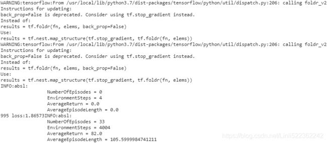
from IPython import display as ipythondisplay
from pyvirtualdisplay import Display

import matplotlib.animation as animation
import matplotlib as mpl
mpl.rc('animation', html='jshtml')

def update_scene( num, frames, patch ):
    patch.set_data( frames[num] )
    return patch,

def plot_animation( frames, repeat=False, interval=40 ):
    fig = plt.figure()
    patch = plt.imshow( frames[0] ) # img
    plt.axis( 'off' )


    anim = animation.FuncAnimation(
            fig,         # figure
            func=update_scene, # The function to call at each frame.
            fargs=(frames, patch), # Additional arguments to pass to each call to func.
            frames = len(frames),  # iterable, int, generator function, or None, optional : Source of data to pass func and each frame of the animation
            repeat=repeat,
            interval=interval
    )
    plt.close()
    return anim
frames = []
def save_frames( trajectory ):
global frames
frames.append( tf_env.pyenv.envs[0].render(mode="rgb_array") )
watch_driver = DynamicStepDriver(
tf_env,
agent.policy,
observers = [ save_frames, ShowProgress(1000) ],
num_steps = 1000
)
final_time_step, final_policy_state = watch_driver.run()
plot_animation(frames)
import PIL
import os

image_path = os.path.join("/content/drive/MyDrive/Colab Notebooks/hand_on_ml", "SpaceInvaders.gif")
frame_images = [ PIL.Image.fromarray(frame) for frame in frames ]
frame_images[0].save( image_path, format='GIF',
                      append_images=frame_images[1:],
                      save_all=True,
                      duration=30,
                      loop=0
                     )