目标检测 YOLO 系列：快速迭代 YOLO v5

目标检测 YOLO 系列：快速迭代 YOLO v5

• 目标检测 YOLO 系列： 开篇
• 目标检测 YOLO 系列： 开宗立派 YOLO v1
• 目标检测 YOLO 系列： 更快更准 YOLO v2
• 目标检测 YOLO 系列： 持续改进 YOLO v3
• 目标检测 YOLO 系列： 你有我有 YOLO v4
• 目标检测 YOLO 系列： 快速迭代 YOLO v5
• 目标检测 YOLO 系列：你有我无 YOLOX

作者：Glenn Jocher
发表时间：2020
Paper 原文：没有发表论文，通过 github（yolov5） 发布。

1. 概览

YOLOv5 刚发布之初还颇有争议，有人觉得它能不能叫 YOLOv5，但是它凭借优秀的性能和完善的工程配套（移植到其他平台）能力，现在（2021年）YOLOv5 依然是检测领域最活跃的模型。YOLOv5 不仅生而不凡，更关键的是它还非常勤快，从发布至今，已经发布了 6 个大版本。所以在使用 YOLOv5 的时候需要注意它的小版本。下面是各个小版本网络结构上的区别

• YOLOv5 6.0

  • 用 conv 替换了 Focus 层

  • 更新了 SPP 和 C3 的结构

• YOLOv5 5.0

  • P5 结构和 4.0 一致

  • P6 4 个输出层（大输入尺寸，stride 分别为 8，16，32，64）

• YOLOv5 4.0

  • 将 YOLOv5 3.0 nn.LeakyReLU(0.1) 和 nn.Hardswish() 替换为 nn.SiLU()

• YOLOv5 3.1

  • 主要是 bug fix

• YOLOv5 3.0

  • 采用 nn.Hardswish() 激活函数

• YOLOv5 2.0

  • 结构不变，主要是 bugfix，但是于 1.0 有兼容性问题

• YOLOv5 1.0

  • 横空出世

除开小版本之外，为了方便进行不同场景下模型的选择，又分为 s, m, l, x 四种不同大小的网络结构。

2. 网络结构

网络结构建议参考 深入浅出Yolo系列之Yolov5核心基础知识完整讲解，里面有高清大图，非常详细。整的来说，相比 v4，主要是加入了 Focus 层，然后激活函数有调整，整体网络架构还是比较类似的。YOLOv5 backbone 可以看做是 modified CSP（CSP 是 YOLOv4 的backbone）。

和 YOLOv4 相比，YOLOv5 在网络结构上改变主要有如下几点：

a. Backbone

• Focus 层。这是 YOLOv5 上新加入的。

• CSP 结构。在 YOLOv4 上，backbone 中也使用了 CSP 结构，但是两者有所区别。
  
  
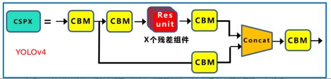
  **b. Neck **

• CSP 结构。Neck 部分 YOLOv4 和 YOLOv5 都采用了 FPN + PAN 的结。但是 Yolov4 的 Neck 结构中，采用的都是普通的卷积操作。而 Yolov5 的 Neck 结构中，采用借鉴 CSPnet 设计的 CSP2 结构，加强网络特征融合的能力。

3. 损失函数

以 5.0 的代码为例，loss 中可以通过设置 fl_gamma 来激活 focal loss。另外 IOU loss 也支持 GIOU， DIOU， CIOU。

def compute_loss(p, targets, model):  # predictions, targets, model
    device = targets.device
    lcls, lbox, lobj = torch.zeros(1, device=device), torch.zeros(1, device=device), torch.zeros(1, device=device)
    tcls, tbox, indices, anchors = build_targets(p, targets, model)  # targets
    h = model.hyp  # hyperparameters

    # Define criteria
    BCEcls = nn.BCEWithLogitsLoss(pos_weight=torch.tensor([h['cls_pw']], device=device))  # weight=model.class_weights)
    BCEobj = nn.BCEWithLogitsLoss(pos_weight=torch.tensor([h['obj_pw']], device=device))

    # Class label smoothing https://arxiv.org/pdf/1902.04103.pdf eqn 3
    cp, cn = smooth_BCE(eps=0.0)

    # Focal loss
    g = h['fl_gamma']  # focal loss gamma
    if g > 0:
        BCEcls, BCEobj = FocalLoss(BCEcls, g), FocalLoss(BCEobj, g)

    # Losses
    nt = 0  # number of targets
    no = len(p)  # number of outputs
    balance = [4.0, 1.0, 0.3, 0.1, 0.03]  # P3-P7
    for i, pi in enumerate(p):  # layer index, layer predictions
        b, a, gj, gi = indices[i]  # image, anchor, gridy, gridx
        tobj = torch.zeros_like(pi[..., 0], device=device)  # target obj

        n = b.shape[0]  # number of targets
        if n:
            nt += n  # cumulative targets
            ps = pi[b, a, gj, gi]  # prediction subset corresponding to targets

            # Regression
            pxy = ps[:, :2].sigmoid() * 2. - 0.5
            pwh = (ps[:, 2:4].sigmoid() * 2) ** 2 * anchors[i]
            pbox = torch.cat((pxy, pwh), 1)  # predicted box
            iou = bbox_iou(pbox.T, tbox[i], x1y1x2y2=False, CIoU=True)  # iou(prediction, target)
            lbox += (1.0 - iou).mean()  # iou loss

            # Objectness
            tobj[b, a, gj, gi] = (1.0 - model.gr) + model.gr * iou.detach().clamp(0).type(tobj.dtype)  # iou ratio

            # Classification
            if model.nc > 1:  # cls loss (only if multiple classes)
                t = torch.full_like(ps[:, 5:], cn, device=device)  # targets
                t[range(n), tcls[i]] = cp
                lcls += BCEcls(ps[:, 5:], t)  # BCE

            # Append targets to text file
            # with open('targets.txt', 'a') as file:
            #     [file.write('%11.5g ' * 4 % tuple(x) + '\n') for x in torch.cat((txy[i], twh[i]), 1)]

        lobj += BCEobj(pi[..., 4], tobj) * balance[i]  # obj loss

    s = 3 / no  # output count scaling
    lbox *= h['box'] * s
    lobj *= h['obj']
    lcls *= h['cls'] * s
    bs = tobj.shape[0]  # batch size

    loss = lbox + lobj + lcls
    return loss * bs, torch.cat((lbox, lobj, lcls, loss)).detach()

4. 后处理

YOLO v5 的后处理代码看起来有点费劲，我整理了一下后处理的流程图，可以作为参考。对于预测出的 xy 值是是相对于输出的 featuremap 的尺寸的，需要结合 stride 转换到相对输入图片尺寸上，而对于 wh 值通过对应的 anchor （注意大的 featuremap 对应小的 anchor）转换到相对于输入图片尺寸上。

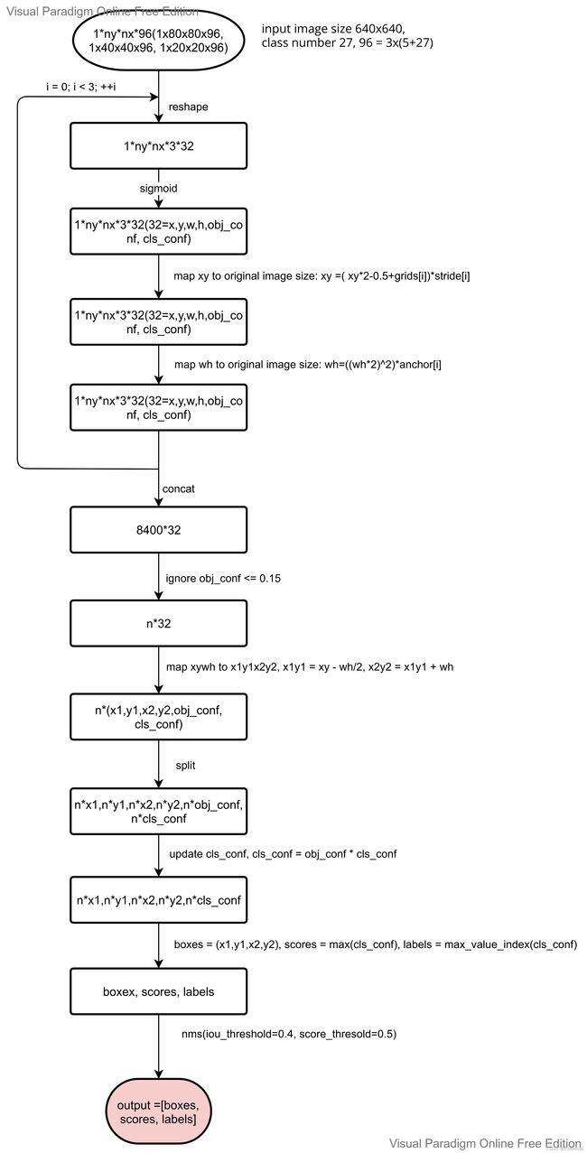
看完后处理，可能有人对下面的两次映射比较疑惑。

 pxy = ps[:, :2].sigmoid() * 2. - 0.5
 pwh = (ps[:, 2:4].sigmoid() * 2) ** 2 * anchors[i]

整理成公式如下：

$$\begin{array}{rl}{b}_x& =2\ast \sigma (t_x)-0.5+c_x\\ b_y& =2\ast \sigma (t_y)-0.5+c_y\\ b_w& =p_w(2\ast \sigma (t_w){)}^2\\ b_h& =p_h(2\ast \sigma (t_h){)}^2\end{array}$$

对于这个问题可以参考下面作者的解释。

• 参考1
• 参考2

5. 性能

YOLO v5 在精度上和 v4 相比可能并没有优势，但是速度（训练和推理，特别是在训练阶段优势明显）上却有很多的优势，另外就是工程化能力也是优势。

参考

• 深入浅出Yolo系列之Yolov5核心基础知识完整讲解