【图像融合】小波变换彩色图像融合（带面板）【含GUI Matlab源码 782期】

⛄一、小波变换彩色图像融合简介

0 引言
目前在各种图像采集与分析系统中已大量使用彩色CCD数码相机, 但是由于其视野有限, 常常获得的只是局部图像, 如果要保证一定的分辨率的前提下采集整体彩色图像, 只能先拍摄具有重叠部分的局部彩色图像, 随后对其进行手工或自动拼接的方法来达到目的。该技术在机器视觉、遥感、虚拟现实、医学图像处理等领域有着广泛的应用。

图像融合包括图像配准和彩色图像融合。目前图像处理软件中比如Photoshop等提供了丰富的处理功能, 以交互方式通过剪切、模糊等操作进行图像拼接, 但由于完全是手工操作, 效率较低且精度不高。然而融合过程完全由计算机自动处理也会遇到难点, 比如进行图像配准的几何变换参数需根据控制点来计算, 所以控制点的准确性对最终配准的精确度会有很大的影响。在人工交互方式下, 控制点是由操作人员仔细观察两幅图像重叠区域的特征而选取出来的, 可信度高, 保证了图像配准的精度, 因此人工交互与计算机自动处理是相辅相成的。图像配准后, 由于当空间三维场景被投影为二维图像时, 场影中的诸多变化因素, 如光照条件、景物遮挡、噪声干扰、景物几何形变和畸变、表面物理特性以及照相机特性等, 都被综合到图像色彩值中, 因此对应同一场景的重叠图像必然存在一定差异。彩色图像融合后, 过渡区的自然平滑是关键。

一种基于小波变换的彩色图像融合算法, 基本步骤是:交互式地在局部图像的重叠部份选取足够多的控制点[1] ―→指定几何变形的类型―→将两幅局部图像变换到同一坐标空间―→色彩空间转换―→小波变换―→对色彩的各分量进行融合―→小波逆变换―→色彩空间转换―→融合图像。考虑到Matlab具有强大、便捷的计算功能, 特别是其丰富的工具箱函数[1], 能极大地提高开发效率, 本文使用Matlab自带的工具箱函数对算法进行了仿真, 由实验可以看出在Matlab这个平台上通过少量编程即可实现复杂算法。

2 基于小波变换的图像融合方法
图像配准之后, 由于局部图像重叠区域之间差异的存在, 如果将图像像素简单叠加, 拼接处就会出现明显的拼接缝。传统的融合方法多是在空间域处理, 没有考虑相应频率域的变化。小波分析具有优良的时频局部性能, 它对信号用一组尺度不同的带通滤波器进行滤波[2], 将信号分解为不同频带进行处理, 能把信号进行多分辨分析, 表达了图像在不同分辨率下的特征, 很适合于图像融合。

设二维尺度函数Φ (x, y) 是可分离的, 相应的尺度函数为Φ (x) , 小波函数为ψ (x) , 即:
Φ (x, y) =Φ (x) Φ (y) (7)
则可构造3个二维基本小函数:
ψ1 (x, y) =Φ (x) ψ (y) (8)
ψ2 (x, y) =ψ (x) Φ (y) (9)
ψ3 (x, y) =ψ (x) ψ (y) (10)
二维小波基可以通过以下伸缩平移实现:

Ψjj,m,n=2-jΨi (2-jx-m, 2-jy-n) (11)
其中j, m, n∈Z, i=1, 2, 3。这样二维图像信号f (x, y) 在尺度2j下的平滑分量 (低频分量) 可用二维序列Dj (m, n) 表示为
Dj (m, n) = (12)
细节成分表示为:
C1j (m, n) = (13)
C2j (m, n) = (14)
C3j (m, n) = (15)
局部图像的重叠区域经过一层二维Mallat算法将得到各自的四个子带图像:LL、LH、HL、HH。图2为基于小波变换的图像融合框图, 首先对重叠区某一色彩分量进行三层小波分解, 然后对色彩不同分量采用不同的融合算法得融合后的系数, 经小波逆变换得融合图像的某一色彩分量。matlab对小波分析提供了全面的支持, 允许用户以图形界面或者命令行形式直接调用小波工具箱函数。例如:idwt2 (dwt2 (image, ‘db2’) , ‘db2’) , 这一行程序先调用dwt2函数对图像image以db2小波进行一层小波变换, 再调用idwt2函数进行小波逆变换, 结果又得到了图像image, matlab的快捷方便可见一斑。

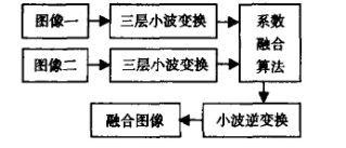
图2 基于小波变换的图像融合框图

⛄二、部分源代码

function varargout = main(varargin)
% MAIN MATLAB code for main.fig
%      MAIN, by itself, creates a new MAIN or raises the existing
%      singleton*.
%
%      H = MAIN returns the handle to a new MAIN or the handle to
%      the existing singleton*.
%
%      MAIN('CALLBACK',hObject,eventData,handles,...) calls the local
%      function named CALLBACK in MAIN.M with the given input arguments.
%
%      MAIN('Property','Value',...) creates a new MAIN or raises the
%      existing singleton*.  Starting from the left, property value pairs are
%      applied to the GUI before main_OpeningFcn gets called.  An
%      unrecognized property name or invalid value makes property application
%      stop.  All inputs are passed to main_OpeningFcn via varargin.
%
%      *See GUI Options on GUIDE's Tools menu.  Choose "GUI allows only one
%      instance to run (singleton)".
%
% See also: GUIDE, GUIDATA, GUIHANDLES

% Edit the above text to modify the response to help main

% Last Modified by GUIDE v2.5 14-Dec-2017 19:28:26

% Begin initialization code - DO NOT EDIT
gui_Singleton = 1;
gui_State = struct('gui_Name',       mfilename, ...
                   'gui_Singleton',  gui_Singleton, ...
                   'gui_OpeningFcn', @main_OpeningFcn, ...
                   'gui_OutputFcn',  @main_OutputFcn, ...
                   'gui_LayoutFcn',  [] , ...
                   'gui_Callback',   []);
if nargin && ischar(varargin{1})
    gui_State.gui_Callback = str2func(varargin{1});
end

if nargout
    [varargout{1:nargout}] = gui_mainfcn(gui_State, varargin{:});
else
    gui_mainfcn(gui_State, varargin{:});
end
% End initialization code - DO NOT EDIT


% --- Executes just before main is made visible.
function main_OpeningFcn(hObject, eventdata, handles, varargin)
% This function has no output args, see OutputFcn.
% hObject    handle to figure
% eventdata  reserved - to be defined in a future version of MATLAB
% handles    structure with handles and user data (see GUIDATA)
% varargin   command line arguments to main (see VARARGIN)

% Choose default command line output for main
handles.output = hObject;
handles.imfusion1=[];
handles.imfusion2=[];
axis(handles.axes1,'off');
axis(handles.axes2,'off');
axis(handles.axes3,'off')
movegui(handles.figure1,'center');
% Update handles structure
guidata(hObject, handles);
uiwait(handles.figure1);

% UIWAIT makes main wait for user response (see UIRESUME)
% uiwait(handles.figure1);


% --- Outputs from this function are returned to the command line.
function varargout = main_OutputFcn(hObject, eventdata, handles) 
% varargout  cell array for returning output args (see VARARGOUT);
% hObject    handle to figure
% eventdata  reserved - to be defined in a future version of MATLAB
% handles    structure with handles and user data (see GUIDATA)

% Get default command line output from handles structure
varargout{1} = handles.output;


% --- Executes on button press in pushbutton1.
function pushbutton1_Callback(hObject, eventdata, handles)
% hObject    handle to pushbutton1 (see GCBO)
% eventdata  reserved - to be defined in a future version of MATLAB
% handles    structure with handles and user data (see GUIDATA)
img =handles.imfusion1;
% img = rgb2gray(img);
% img = img(20:160,140:280);
nn=10;
img=imresize(img,[58*nn 77*nn]);


img2 =handles.imfusion2;
% img2 = rgb2gray(img2);
% img2 = img2(20:160,140:280);
img2=imresize(img2,[58*nn 77*nn]);
[RcA1,RcH1,RcV1,RcD1] = dwt2(img,'sym4');%LL1,HL1,LH1,HH1
[VcA1,VcH1,VcV1,VcD1] = dwt2(img2,'sym4');%LL1,HL1,LH1,HH1
[RcA2,RcH2,RcV2,RcD2] = dwt2(RcA1,'sym4');%LL1,HL1,LH1,HH1
[VcA2,VcH2,VcV2,VcD2] = dwt2(VcA1,'sym4');%LL1,HL1,LH1,HH1
%%%%%% 2级小波融合
%%%%%% 策略1：  低频平均；高频模值较大者
[M1,N1,P1] = size(RcA1);
[M2,N2,P2] = size(RcA2);
%%%%%%1级
cA10 = (RcA1 + VcA1)*0.5;
for i=1:M1
    for j=1:N1
        for k=1:3
        if abs(RcH1(i,j,k)) > abs(VcH1(i,j,k))
              cH10(i,j,k) = RcH1(i,j,k);      
        else
              cH10(i,j,k) = VcH1(i,j,k); 
        end
        if abs(RcV1(i,j,k)) > abs(VcV1(i,j,k))
              cV10(i,j,k) = RcV1(i,j,k);      
        else
              cV10(i,j,k) = VcV1(i,j,k); 
        end
        if abs(RcD1(i,j,k)) > abs(VcD1(i,j,k))
              cD10(i,j,k) = RcD1(i,j,k);      
        else
              cD10(i,j,k) = VcD1(i,j,k); 
        end        
        end
    end
end
%%%%%%%2级
cA20 = (RcA2 + VcA2)*0.5;
for i=1:M2
    for j=1:N2
        for k=1:3
        if abs(RcH2(i,j,k)) > abs(VcH2(i,j,k))
              cH20(i,j,k) = RcH2(i,j,k);      
        else
              cH20(i,j,k) = VcH2(i,j,k); 
        end
        if abs(RcV2(i,j,k)) > abs(VcV2(i,j,k))
              cV20(i,j,k) = RcV2(i,j,k);      
        else
              cV20(i,j,k) = VcV2(i,j,k); 
        end
        if abs(RcD2(i,j,k)) > abs(VcD2(i,j,k))
              cD20(i,j,k) = RcD2(i,j,k);      
        else
              cD20(i,j,k) = VcD2(i,j,k); 
        end        
        end
    end
end
%%%%%%反变换
img_fuse2 = idwt2(cA20,cH20,cV20,cD20,'sym4');%LL1,HL1,LH1,HH1
img_fuse2 = img_fuse2(1:M1,1:N1,1:3);
img_fuse0 = idwt2(img_fuse2,cH10,cV10,cD10,'sym4');
for k=1:3
%     a=max(max(img_fuse0(:,:,k)));
%     b=min(min(img_fuse0(:,:,k)));
%     img_fuse0(:,:,k)=1/(b-a)*img_fuse0(:,:,k)-(1/(b-a)*a);
a=max(max(img_fuse0(:,:,k)));
 img_fuse0(:,:,k)= img_fuse0(:,:,k)./a;
end
axes(handles.axes3);
imshow(img_fuse0);
guidata(hObject, handles);
 

## ⛄三、运行结果
![在这里插入图片描述](https://img-blog.csdnimg.cn/2ea1c48e75cb432590483cd8e786e500.png?x-oss-process=image/watermark,type_d3F5LXplbmhlaQ,shadow_50,text_Q1NETiBA57Sr5p6B56We5YWJ,size_20,color_FFFFFF,t_70,g_se,x_16#pic_center)

## ⛄四、matlab版本及参考文献
**1 matlab版本**
2014a

**2 参考文献**
[1]汪强,尹峰,刘钢钦.基于小波的彩色图像融合技术[M].计算机仿真. 2005,(11)

**3 备注**
简介此部分摘自互联网，仅供参考，若侵权，联系删除