高光谱图像分类

高光谱图像分类

本次作业参考论文《HybridSN: Exploring 3-D–2-DCNN Feature Hierarchy for Hyperspectral Image Classification》完成，使用HybridSN模型进行高光谱图像分类（HSI），并尝试引入注意力机制来优化分类结果。3D卷积和2D卷积的区别在于3D卷积比2D卷积多一个深度信息，2D卷积可以认为是深度为1的3D卷积，在PyTorch网络骨架里的区别是，3D卷积shape为(batch_size,channel,depth,height,weight)，2D卷积 shape为(batch_size,channel,height,weight)。传统的二维CNN中，卷积只应用在空间维度上，覆盖上一层的所有特征图，来计算二维判别特征图。HSI分类问题，希望能够同时捕获多个波段编码的光谱信息和空间信息。二维CNN不能处理光谱信息，而三维CNN可以在HSI数据中同时提取光谱和空间特征，但是代价是增加了计算复杂度。论文中提到，高光谱图像是立体数据，也有光谱维数，仅凭2D-CNN无法从光谱维度中提取出具有良好鉴别能力的feature maps，3D-CNN在计算上更加复杂，对于在许多光谱带上具有相似纹理的类来说，单独使用也不会有很好的效果，混合CNN模型克服了之前模型的缺点，将3D-CNN和2D-CNN层组合到该模型中，充分利用光谱和空间特征图，以达到最大可能的精度。下面开始介绍论文中提到的HybridSN模型：

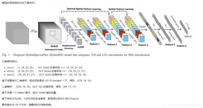
1.构建HybridSN模型

class HybridSN(nn.Module):
  def __init__(self):
    super(HybridSN,self).__init__()
    self.conv3d_1=nn.Sequential(
        nn.Conv3d(1,8,kernel_size=(7,3,3),stride=1,padding=0),
        nn.BatchNorm3d(8),
        nn.ReLU(inplace=True),
    )
    self.conv3d_2 = nn.Sequential(
        nn.Conv3d(8, 16, kernel_size=(5, 3, 3), stride=1, padding=0),
        nn.BatchNorm3d(16),
        nn.ReLU(inplace = True),
    ) 
    self.conv3d_3 = nn.Sequential(
        nn.Conv3d(16, 32, kernel_size=(3, 3, 3), stride=1, padding=0),
        nn.BatchNorm3d(32),
        nn.ReLU(inplace = True)
    )

    self.conv2d = nn.Sequential(
        nn.Conv2d(576, 64, kernel_size=(3, 3), stride=1, padding=0),
        nn.BatchNorm2d(64),
        nn.ReLU(inplace = True),
    )
    self.fc1 = nn.Linear(18496,256)
    self.fc2 = nn.Linear(256,128)
    self.fc3 = nn.Linear(128,16)
    self.dropout = nn.Dropout(p = 0.4)

  def forward(self,x):
    out = self.conv3d_1(x)
    out = self.conv3d_2(out)
    out = self.conv3d_3(out)
    out = self.conv2d(out.reshape(out.shape[0],-1,19,19))
    out = out.reshape(out.shape[0],-1)
    out = F.relu(self.dropout(self.fc1(out)))
    out = F.relu(self.dropout(self.fc2(out)))
    out = self.fc3(out)
    return out

2.创建数据集

首先对高光谱数据实施PCA降维；然后创建 keras 方便处理的数据格式；然后随机抽取 10% 数据做为训练集，剩余的做为测试集。

# 对高光谱数据 X 应用 PCA 变换
def applyPCA(X, numComponents):
    newX = np.reshape(X, (-1, X.shape[2]))
    pca = PCA(n_components=numComponents, whiten=True)
    newX = pca.fit_transform(newX)
    newX = np.reshape(newX, (X.shape[0], X.shape[1], numComponents))
    return newX

# 对单个像素周围提取 patch 时，边缘像素就无法取了，因此，给这部分像素进行 padding 操作
def padWithZeros(X, margin=2):
    newX = np.zeros((X.shape[0] + 2 * margin, X.shape[1] + 2* margin, X.shape[2]))
    x_offset = margin
    y_offset = margin
    newX[x_offset:X.shape[0] + x_offset, y_offset:X.shape[1] + y_offset, :] = X
    return newX

# 在每个像素周围提取 patch ，然后创建成符合 keras 处理的格式
def createImageCubes(X, y, windowSize=5, removeZeroLabels = True):
    # 给 X 做 padding
    margin = int((windowSize - 1) / 2)
    zeroPaddedX = padWithZeros(X, margin=margin)
    # split patches
    patchesData = np.zeros((X.shape[0] * X.shape[1], windowSize, windowSize, X.shape[2]))
    patchesLabels = np.zeros((X.shape[0] * X.shape[1]))
    patchIndex = 0
    for r in range(margin, zeroPaddedX.shape[0] - margin):
        for c in range(margin, zeroPaddedX.shape[1] - margin):
            patch = zeroPaddedX[r - margin:r + margin + 1, c - margin:c + margin + 1]   
            patchesData[patchIndex, :, :, :] = patch
            patchesLabels[patchIndex] = y[r-margin, c-margin]
            patchIndex = patchIndex + 1
    if removeZeroLabels:
        patchesData = patchesData[patchesLabels>0,:,:,:]
        patchesLabels = patchesLabels[patchesLabels>0]
        patchesLabels -= 1
    return patchesData, patchesLabels

def splitTrainTestSet(X, y, testRatio, randomState=345):
    X_train, X_test, y_train, y_test = train_test_split(X, y, test_size=testRatio, random_state=randomState, stratify=y)
    return X_train, X_test, y_train, y_test
# 地物类别
class_num = 16
X = sio.loadmat('Indian_pines_corrected.mat')['indian_pines_corrected']
y = sio.loadmat('Indian_pines_gt.mat')['indian_pines_gt']

# 用于测试样本的比例
test_ratio = 0.90
# 每个像素周围提取 patch 的尺寸
patch_size = 25
# 使用 PCA 降维，得到主成分的数量
pca_components = 30

print('Hyperspectral data shape: ', X.shape)
print('Label shape: ', y.shape)

print('\n... ... PCA tranformation ... ...')
X_pca = applyPCA(X, numComponents=pca_components)
print('Data shape after PCA: ', X_pca.shape)

print('\n... ... create data cubes ... ...')
X_pca, y = createImageCubes(X_pca, y, windowSize=patch_size)
print('Data cube X shape: ', X_pca.shape)
print('Data cube y shape: ', y.shape)

print('\n... ... create train & test data ... ...')
Xtrain, Xtest, ytrain, ytest = splitTrainTestSet(X_pca, y, test_ratio)
print('Xtrain shape: ', Xtrain.shape)
print('Xtest  shape: ', Xtest.shape)

# 改变 Xtrain, Ytrain 的形状，以符合 keras 的要求
Xtrain = Xtrain.reshape(-1, patch_size, patch_size, pca_components, 1)
Xtest  = Xtest.reshape(-1, patch_size, patch_size, pca_components, 1)
print('before transpose: Xtrain shape: ', Xtrain.shape) 
print('before transpose: Xtest  shape: ', Xtest.shape) 

# 为了适应 pytorch 结构，数据要做 transpose
Xtrain = Xtrain.transpose(0, 4, 3, 1, 2)
Xtest  = Xtest.transpose(0, 4, 3, 1, 2)
print('after transpose: Xtrain shape: ', Xtrain.shape) 
print('after transpose: Xtest  shape: ', Xtest.shape) 


""" Training dataset"""
class TrainDS(torch.utils.data.Dataset): 
    def __init__(self):
        self.len = Xtrain.shape[0]
        self.x_data = torch.FloatTensor(Xtrain)
        self.y_data = torch.LongTensor(ytrain)        
    def __getitem__(self, index):
        # 根据索引返回数据和对应的标签
        return self.x_data[index], self.y_data[index]
    def __len__(self): 
        # 返回文件数据的数目
        return self.len

""" Testing dataset"""
class TestDS(torch.utils.data.Dataset): 
    def __init__(self):
        self.len = Xtest.shape[0]
        self.x_data = torch.FloatTensor(Xtest)
        self.y_data = torch.LongTensor(ytest)
    def __getitem__(self, index):
        # 根据索引返回数据和对应的标签
        return self.x_data[index], self.y_data[index]
    def __len__(self): 
        # 返回文件数据的数目
        return self.len

# 创建 trainloader 和 testloader
trainset = TrainDS()
testset  = TestDS()
train_loader = torch.utils.data.DataLoader(dataset=trainset, batch_size=128, shuffle=True, num_workers=2)
test_loader  = torch.utils.data.DataLoader(dataset=testset,  batch_size=128, shuffle=False, num_workers=2)

运行结果

3.开始训练

device = torch.device("cuda:0" if torch.cuda.is_available() else "cpu")

# 网络放到GPU上
net = HybridSN().to(device)
criterion = nn.CrossEntropyLoss()
optimizer = optim.Adam(net.parameters(), lr=0.001)

# 开始训练
total_loss = 0
for epoch in range(100):
    for i, (inputs, labels) in enumerate(train_loader):
        inputs = inputs.to(device)
        labels = labels.to(device)
        # 优化器梯度归零
        optimizer.zero_grad()
        # 正向传播 +　反向传播 + 优化 
        outputs = net(inputs)
        loss = criterion(outputs, labels)
        loss.backward()
        optimizer.step()
        total_loss += loss.item()
    print('[Epoch: %d]   [loss avg: %.4f]   [current loss: %.4f]' %(epoch + 1, total_loss/(epoch+1), loss.item()))

print('Finished Training')

运行结果

3.模型测试

count = 0
# 模型测试
for inputs, _ in test_loader:
    inputs = inputs.to(device)
    outputs = net(inputs)
    outputs = np.argmax(outputs.detach().cpu().numpy(), axis=1)
    if count == 0:
        y_pred_test =  outputs
        count = 1
    else:
        y_pred_test = np.concatenate( (y_pred_test, outputs) )

# 生成分类报告
classification = classification_report(ytest, y_pred_test, digits=4)
print(classification)

运行结果

准确率达到了97.67%。关于为什么多次训练网络，会发现每次分类的结果都不一样，是因为网络的全连接层中为了避免过拟合使用了 nn.Dropout(p=0.4)，训练模式下是启用 Dropout和BN 层(本例没有)的，网络层的节点会随机失活。原始的代码没有注意到pytorch模型网络的训练模式和测试模式即 net.train() 和 net.eval() (这里net是我们构建的HybirdSN)，在测试时仍然采用训练模式，导致每次测试分类结果不一样。如果测试时启用net.eval()就会得到相同的分类结果。

4.备用函数以及分类结果

from operator import truediv

def AA_andEachClassAccuracy(confusion_matrix):
    counter = confusion_matrix.shape[0]
    list_diag = np.diag(confusion_matrix)
    list_raw_sum = np.sum(confusion_matrix, axis=1)
    each_acc = np.nan_to_num(truediv(list_diag, list_raw_sum))
    average_acc = np.mean(each_acc)
    return each_acc, average_acc


def reports (test_loader, y_test, name):
    count = 0
    # 模型测试
    for inputs, _ in test_loader:
        inputs = inputs.to(device)
        outputs = net(inputs)
        outputs = np.argmax(outputs.detach().cpu().numpy(), axis=1)
        if count == 0:
            y_pred =  outputs
            count = 1
        else:
            y_pred = np.concatenate( (y_pred, outputs) )

    if name == 'IP':
        target_names = ['Alfalfa', 'Corn-notill', 'Corn-mintill', 'Corn'
                        ,'Grass-pasture', 'Grass-trees', 'Grass-pasture-mowed', 
                        'Hay-windrowed', 'Oats', 'Soybean-notill', 'Soybean-mintill',
                        'Soybean-clean', 'Wheat', 'Woods', 'Buildings-Grass-Trees-Drives',
                        'Stone-Steel-Towers']
    elif name == 'SA':
        target_names = ['Brocoli_green_weeds_1','Brocoli_green_weeds_2','Fallow','Fallow_rough_plow','Fallow_smooth',
                        'Stubble','Celery','Grapes_untrained','Soil_vinyard_develop','Corn_senesced_green_weeds',
                        'Lettuce_romaine_4wk','Lettuce_romaine_5wk','Lettuce_romaine_6wk','Lettuce_romaine_7wk',
                        'Vinyard_untrained','Vinyard_vertical_trellis']
    elif name == 'PU':
        target_names = ['Asphalt','Meadows','Gravel','Trees', 'Painted metal sheets','Bare Soil','Bitumen',
                        'Self-Blocking Bricks','Shadows']
    
    classification = classification_report(y_test, y_pred, target_names=target_names)
    oa = accuracy_score(y_test, y_pred)
    confusion = confusion_matrix(y_test, y_pred)
    each_acc, aa = AA_andEachClassAccuracy(confusion)
    kappa = cohen_kappa_score(y_test, y_pred)
    
    return classification, confusion, oa*100, each_acc*100, aa*100, kappa*100
classification, confusion, oa, each_acc, aa, kappa = reports(test_loader, ytest, 'IP')
classification = str(classification)
confusion = str(confusion)
file_name = "classification_report.txt"

with open(file_name, 'w') as x_file:
    x_file.write('\n')
    x_file.write('{} Kappa accuracy (%)'.format(kappa))
    x_file.write('\n')
    x_file.write('{} Overall accuracy (%)'.format(oa))
    x_file.write('\n')
    x_file.write('{} Average accuracy (%)'.format(aa))
    x_file.write('\n')
    x_file.write('\n')
    x_file.write('{}'.format(classification))
    x_file.write('\n')
    x_file.write('{}'.format(confusion))
# load the original image
X = sio.loadmat('Indian_pines_corrected.mat')['indian_pines_corrected']
y = sio.loadmat('Indian_pines_gt.mat')['indian_pines_gt']

height = y.shape[0]
width = y.shape[1]

X = applyPCA(X, numComponents= pca_components)
X = padWithZeros(X, patch_size//2)

# 逐像素预测类别
outputs = np.zeros((height,width))
for i in range(height):
    for j in range(width):
        if int(y[i,j]) == 0:
            continue
        else :
            image_patch = X[i:i+patch_size, j:j+patch_size, :]
            image_patch = image_patch.reshape(1,image_patch.shape[0],image_patch.shape[1], image_patch.shape[2], 1)
            X_test_image = torch.FloatTensor(image_patch.transpose(0, 4, 3, 1, 2)).to(device)                                   
            prediction = net(X_test_image)
            prediction = np.argmax(prediction.detach().cpu().numpy(), axis=1)
            outputs[i][j] = prediction+1
    if i % 20 == 0:
        print('... ... row ', i, ' handling ... ...')
predict_image = spectral.imshow(classes = outputs.astype(int),figsize =(5,5))

分类结果

我测试了很多次都是这个结果，这个结果并没有达到预期。

5.往模型中添加注意力机制

修改后的模型如下（其余代码并没有大的改动）：

# 通道注意力机制
class ChannelAttention(nn.Module):
    def __init__(self, in_planes, ratio=16):
        super(ChannelAttention, self).__init__()
        self.avg_pool = nn.AdaptiveAvgPool2d(1)
        self.max_pool = nn.AdaptiveMaxPool2d(1)
 
        self.fc1   = nn.Conv2d(in_planes, in_planes // 16, 1, bias=False)
        self.relu1 = nn.ReLU()
        self.fc2   = nn.Conv2d(in_planes // 16, in_planes, 1, bias=False)
 
        self.sigmoid = nn.Sigmoid()
 
    def forward(self, x):
        avg_out = self.fc2(self.relu1(self.fc1(self.avg_pool(x))))
        max_out = self.fc2(self.relu1(self.fc1(self.max_pool(x))))
        out = avg_out + max_out
        return self.sigmoid(out)
# 空间注意力机制
class SpatialAttention(nn.Module):
    def __init__(self, kernel_size=7):
        super(SpatialAttention, self).__init__()
 
        assert kernel_size in (3, 7), 'kernel size must be 3 or 7'
        padding = 3 if kernel_size == 7 else 1
 
        self.conv1 = nn.Conv2d(2, 1, kernel_size, padding=padding, bias=False)
        self.sigmoid = nn.Sigmoid()
 
    def forward(self, x):
        avg_out = torch.mean(x, dim=1, keepdim=True)
        max_out, _ = torch.max(x, dim=1, keepdim=True)
        x = torch.cat([avg_out, max_out], dim=1)
        x = self.conv1(x)
        return self.sigmoid(x)
 
# 网络骨架
class HybridSN(nn.Module):
    def __init__(self, num_classes, self_attention=False):
        super(HybridSN, self).__init__()
        # out = (width - kernel_size + 2*padding)/stride + 1
        # => padding = ( stride * (out-1) + kernel_size - width)
        # 这里因为 stride == 1 所有卷积计算得到的padding都为 0
 
        #默认不使用注意力机制
        self.self_attention = self_attention
 
        # 3D卷积块
        self.block_1_3D = nn.Sequential(
            nn.Conv3d(
                in_channels=1,
                out_channels=8,
                kernel_size=(7, 3, 3),
                stride=1,
                padding=0
            ),
            nn.ReLU(inplace=True),
            nn.Conv3d(
                in_channels=8,
                out_channels=16,
                kernel_size=(5, 3, 3),
                stride=1,
                padding=0
            ),
            nn.ReLU(inplace=True),
            nn.Conv3d(
                in_channels=16,
                out_channels=32,
                kernel_size=(3, 3, 3),
                stride=1,
                padding=0
            ),
            nn.ReLU(inplace=True)
        )
       
        if self_attention:
            self.channel_attention_1 = ChannelAttention(576)
            self.spatial_attention_1 = SpatialAttention(kernel_size=7)
 
        # 2D卷积块
        self.block_2_2D = nn.Sequential(
            nn.Conv2d(
                in_channels=576,
                out_channels=64,
                kernel_size=(3, 3)
            ),
            nn.ReLU(inplace=True)
        )
 
        if self_attention:
            self.channel_attention_2 = ChannelAttention(64)
            self.spatial_attention_2 = SpatialAttention(kernel_size=7)
 
        # 全连接层
        self.classifier = nn.Sequential(
            nn.Linear(
                in_features=18496,
                out_features=256
            ),
            nn.Dropout(p=0.4),
            nn.Linear(
                in_features=256,
                out_features=128
            ),
            nn.Dropout(p=0.4),
            nn.Linear(
                in_features=128,
                out_features=num_classes
            )
            # pytorch交叉熵损失函数是混合了softmax的。不需要再使用softmax
        )
    def forward(self, x):
        y = self.block_1_3D(x)
        y = y.view(-1, y.shape[1] * y.shape[2], y.shape[3], y.shape[4])
        if self.self_attention:
            y = self.channel_attention_1(y) * y
            y = self.spatial_attention_1(y) * y
        y = self.block_2_2D(y)
        if self.self_attention:
            y = self.channel_attention_2(y) * y
            y = self.spatial_attention_2(y) * y
 
        y = y.view(y.size(0), -1)
 
        y = self.classifier(y)
        return y

模型测试结果

分类结果

从测试结果来看，准确率是96.25%，反而降低了，但是分类结果达到了我预期的效果。

5.如何通过注意力机制增强模型分类性能？

如果从维度上考虑，可以从图像空间、通道和光谱的波长三个方向使用注意力机制来处理特征，可能会取得更好的分类效果。

高光谱图像的特征中，局部关键性区域往往集中在某小块区域，局部特征的提取仅与这一小块相关，如果模型在全部特征向量上进行特征提取，可能由于特征向量中存在某些不相关区域而导致次优结果。采用空间注意力，找到与局部特征相关的特征空间，然后从该特征空间进行特征提取会提取到比较准确的特征。