【雷达通信】SAR雷达系统反设计及典型目标建模与仿真实现研究——目标生成与检测（Matlab代码实现）

 ‍个人主页：研学社的博客 

欢迎来到本博客❤️❤️

博主优势：博客内容尽量做到思维缜密，逻辑清晰，为了方便读者。

⛳️座右铭：行百里者，半于九十。

本文目录如下：

1 概述

现代战争对雷达目标识别提出了更高的要求,由于现役雷达大部分是低分辨雷达,对其开展目标识别技术的研究具有重要军事意义。在小样本、样本不均衡等复杂电磁环境条件下,传统低分辨雷达目标识别方法存在泛化性较差、识别率较低等问题。本文围绕深度学习方法对低分辨雷达目标识别技术开展研究,主要研究内容如下:传统低分辨雷达目标识别技术采用先提取信号特征,再基于特征进行识别的两步识别方法。
 

2 运行结果

 

 

部分代码：

%% Signal generation and Moving Target simulation
% Running the radar scenario over the time. 

for i=1:length(t)         
  % *%TODO* 
  %For each time stamp update the Range of the Target for constant velocity. 
  r_t(i) = range + (vel*t(i));
  td(i) = (2 * r_t(i)) / c;

  % *%TODO* :
  %For each time sample we need update the transmitted and
  %received signal. 

  Tx(i)   = cos(2*pi*(fc*t(i) + (slope*t(i)^2)/2 ) );
  Rx(i)   = cos(2*pi*(fc*(t(i) -td(i)) + (slope * (t(i)-td(i))^2)/2 ) );
    
  % *%TODO* :
  %Now by mixing the Transmit and Receive generate the beat signal
  %This is done by element wise matrix multiplication of Transmit and
  %Receiver Signal

  Mix(i) = Tx(i) .* Rx(i);
end

%% RANGE MEASUREMENT

 % *%TODO* :
%reshape the vector into Nr*Nd array. Nr and Nd here would also define the size of
%Range and Doppler FFT respectively.
Mix = reshape(Mix, [Nr, Nd]);

 % *%TODO* :
%run the FFT on the beat signal along the range bins dimension (Nr) and
%normalize.
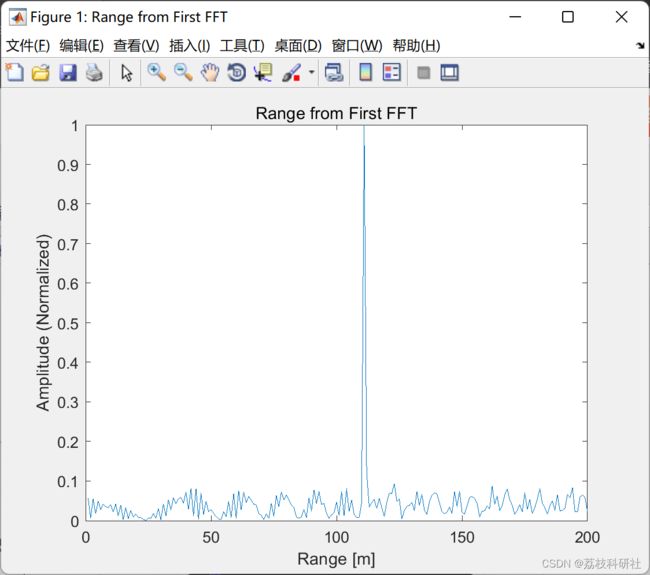
signal_fft = fft(Mix, Nr);

 % *%TODO* :
% Take the absolute value of FFT output
signal_fft = abs(signal_fft);
signal_fft = signal_fft ./ max(signal_fft); % Normalize

 % *%TODO* :
% Output of FFT is double sided signal, but we are interested in only one side of the spectrum.
% Hence we throw out half of the samples.
signal_fft = signal_fft(1 : Nr/2-1);

%plotting the range
figure ('Name','Range from First FFT')
% *%TODO* :
% plot FFT output 
plot(signal_fft);
axis ([0 180 0 1]);
title('Range from First FFT');
ylabel('Amplitude (Normalized)');
xlabel('Range [m]');
axis ([0 200 0 1]);

%% RANGE DOPPLER RESPONSE
% The 2D FFT implementation is already provided here. This will run a 2DFFT
% on the mixed signal (beat signal) output and generate a range doppler
% map.You will implement CFAR on the generated RDM

% Range Doppler Map Generation.
% The output of the 2D FFT is an image that has reponse in the range and
% doppler FFT bins. So, it is important to convert the axis from bin sizes
% to range and doppler based on their Max values.

Mix=reshape(Mix,[Nr,Nd]);

% 2D FFT using the FFT size for both dimensions.
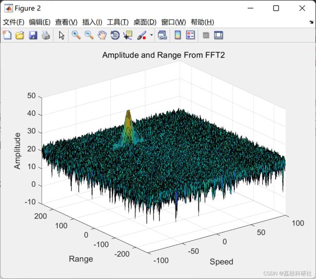
signal_fft2 = fft2(Mix,Nr,Nd);

% Taking just one side of signal from Range dimension.
signal_fft2 = signal_fft2(1:Nr/2,1:Nd);
signal_fft2 = fftshift (signal_fft2);

RDM = abs(signal_fft2);
RDM = 10*log10(RDM) ;

%use the surf function to plot the output of 2DFFT and to show axis in both
%dimensions

doppler_axis = linspace(-100,100,Nd);
range_axis = linspace(-200,200,Nr/2)*((Nr/2)/400);

figure,surf(doppler_axis,range_axis,RDM);
title('Amplitude and Range From FFT2');
xlabel('Speed');
ylabel('Range');
zlabel('Amplitude');

%% CFAR implementation

%Slide Window through the complete Range Doppler Map

% *%TODO* :
%Select the number of Training Cells in both the dimensions.
n_train_cells = 10;
n_train_bands = 8;

% *%TODO* :
%Select the number of Guard Cells in both dimensions around the Cell under 
%test (CUT) for accurate estimation
n_guard_cells = 4;
n_guard_bands = 4;

% *%TODO* :
% offset the threshold by SNR value in dB
offset = 1.4;

% *%TODO* :
%Create a vector to store noise_level for each iteration on training cells
noise_level = zeros(1,1);

% *%TODO* :
%design a loop such that it slides the CUT across range doppler map by
%giving margins at the edges for Training and Guard Cells.
%For every iteration sum the signal level within all the training
%cells. To sum convert the value from logarithmic to linear using db2pow
%function. Average the summed values for all of the training%cells used. After averaging convert it back to logarithimic using pow2db.
%Further add the offset to it to determine the threshold. Next, compare the
%signal under CUT with this threshold. If the CUT level > threshold assign
%it a value of 1, else equate it to 0.

   % Use RDM[x,y] as the matrix from the output of 2D FFT for implementing
   % CFAR

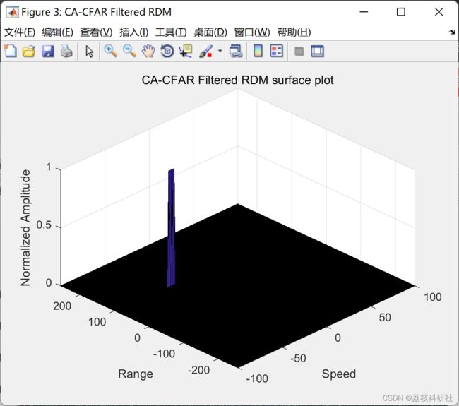
RDM = RDM / max(RDM(:));

for row0 = n_train_cells + n_guard_cells + 1 : (Nr/2) - (n_train_cells + n_guard_cells)
  for col0 = n_train_bands + n_guard_bands + 1 : (Nd) - (n_train_bands + n_guard_bands)
    %Create a vector to store noise_level for each iteration on training cells
    noise_level = zeros(1, 1);

    for row1 = row0 - (n_train_cells + n_guard_cells) : row0 + (n_train_cells + n_guard_cells)
      for col1 = col0 - (n_train_bands + n_guard_bands) : col0 + (n_train_bands + n_guard_bands)
        if (abs(row0 - row1) > n_guard_cells || abs(col0 - col1) > n_guard_bands)
          noise_level = noise_level + db2pow(RDM(row1, col1));
        end
      end
    end

    % Calculate threshold from noise average then add the offset
    thresh = pow2db(noise_level / (2 * (n_train_bands + n_guard_bands + 1) * 2 * (n_train_cells + n_guard_cells + 1) - (n_guard_cells * n_guard_bands) - 1));
    thresh = thresh + offset;

    CUT = RDM(row1,col1);

    if (CUT < thresh)
      RDM(row0, col0) = 0;
    else
      RDM(row0, col0) = 1;
    end

  end
end

% *%TODO* :
% The process above will generate a thresholded block, which is smaller 
%than the Range Doppler Map as the CUT cannot be located at the edges of
%matrix. Hence,few cells will not be thresholded. To keep the map size same
% set those values to 0. 
 
RDM(RDM~=0 & RDM~=1) = 0;

% *%TODO* :
%display the CFAR output using the Surf function like we did for Range
%Doppler Response output.
figure('Name', 'CA-CFAR Filtered RDM')
surf(doppler_axis, range_axis, RDM);
%colorbar;
title( 'CA-CFAR Filtered RDM surface plot');
xlabel('Speed');
ylabel('Range');
zlabel('Normalized Amplitude');
view(315, 45);

 

3 Matlab代码实现

4 参考文献

部分理论来源于网络，如有侵权请联系删除。

[1]易重辉. 基于深度学习的低空监视雷达目标检测的研究[D].四川大学,2021.DOI:10.27342/d.cnki.gscdu.2021.000528.