李宏毅作业十二 Transfer Learning（迁移学习）

系列文章目录

李宏毅作业十 Generative Adversarial Network生成对抗网络(代码)
李宏毅作业九 Anomaly Detection异常检测
李宏毅作业八unsupervised无监督聚类学习
李宏毅作业七其三 Network Compression (Network Pruning)
李宏毅作业七其二 Network Compression (Knowledge Distillation)
李宏毅作业七其一 Network Compression (Architecuture Design)
李宏毅作业六 Adversarial Attack对抗攻击

---

前言

• 本篇博客相较之前将做出一定改进，会放出实验结果（花在写博客的时间又要增加了--），也是方便我自己回头回顾。
• 我也会着重写上理论知识，但侧重点还在于代码，不过不会像之前一带而过了。
• 本片代码我不多注释了，因为我前面几篇代码已经注释的很详细了。基本可以无障碍浏览代码。

提示：以下是本篇文章正文内容，下面案例可供参考

一、Transfer Learning

1.任务

迁移学习主要是将已有数据的领域知识迁移到数据缺乏的领域任务中。

今天我们主要做的是Domain Adversarial Training，对抗性领域训练。

在对抗性领域训练中，由于源数据域是有标签的，而目标数据域是没有标签的。那么在我们训练的过程中，由于特征提取模块只见过源数据域，没见过目标数据域，很容易导致目标数据域的特征被当作异常特征对待。

2.方法

针对这个问题，课程里给出的方法是将目标数据和源数据经过特征提取模块
后提取的特征放入同一个特征分布器上。

• 下面是Domain Adversarial Training of Nerural Networks (DaNN)
  
• 在后面追加一个Domain Classifier,在学习过程中，让Domain Classifier去判断上面特征提取模块提取的特征来源哪个数据集，接着让特征提取模块学习产生特征来骗过Domain Classifier。

这样，特征提取模块提取的特征的泛化性和适用性才会更好。

示例：pandas 是基于NumPy 的一种工具，该工具是为了解决数据分析任务而创建的。

二、代码实现

这部分代码主要实现的是通过10类的图片（源数据）来对涂鸦画（目标数据）进行分类。

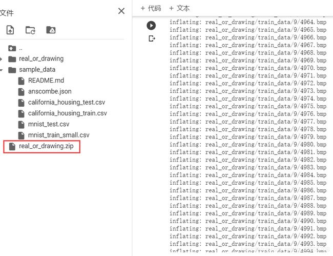
1.下载数据集

# Download dataset
!gdown --id '12-07DSquGdzN3JBHBChN4nMo3i8BqTiL' --output real_or_drawing.zip
# Unzip the files
!unzip real_or_drawing.zip

由于我这是重复下载，所以我直接填的N，直接跳过。
正常如下：

2.1查看数据集

import matplotlib.pyplot as plt

def no_axis_show(img, title='', cmap=None):
  # imshow, 縮放模式為nearest。
  fig = plt.imshow(img, interpolation='nearest', cmap=cmap)
  # 不要顯示axis。
  fig.axes.get_xaxis().set_visible(False)
  fig.axes.get_yaxis().set_visible(False)
  plt.title(title)

titles = ['horse', 'bed', 'clock', 'apple', 'cat', 'plane', 'television', 'dog', 'dolphin', 'spider']
plt.figure(figsize=(18, 18))
for i in range(10):
  plt.subplot(1, 10, i+1)
  fig = no_axis_show(plt.imread(f'real_or_drawing/train_data/{i}/{500*i}.bmp'), title=titles[i])

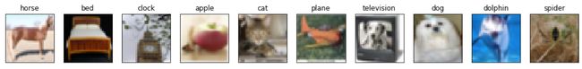
我们可以看到有10类。在最终生成的CSV文件上，你打开也可以看到label分为10类，不过以0~ 9表示。

3.授权Google Drive File Stream

from google.colab import drive#授权Google Drive File Stream访问你的谷歌硬盘
drive.mount('/content/drive')

这步会跳转一个界面，授权会得到授权码，复制粘贴回来即可。

2.2查看数据集

plt.figure(figsize=(18, 18))
for i in range(20):
  plt.subplot(2, 10, i+1)
  fig = no_axis_show(plt.imread(f'real_or_drawing/test_data/0/' + str(i).rjust(5, '0') + '.bmp'))

4.Special Domain Knowledge

• Canny Edge Detection
  cv2.Canny使用非常方便，只需要两个参数: low_threshold, high_threshold。

cv2.Canny(image, low_threshold, high_threshold)
参数：images 图片
low_threshold,边缘低阈值（超过低阈值，需要再判断一下，才能确定是否为边缘）
high_threshold，边缘高阈值（超过高阈值，直接判定为边缘）

• 这里为什么要用到 Canny Edge Detection 呢？
• 在前面显示数据集我们可以看到目标数据和源数据在边界上有着共同点，即使内部像素不一致，在人眼里仅仅通过边缘还是可以分辨出来的。所以这次迁移学习我们将从边缘下手。
• 所以具体情况具体分析，这次迁移学习通过抓住两个数据的共同点来进行训练。

代码

代码如下：

import cv2
import matplotlib.pyplot as plt
titles = ['horse', 'bed', 'clock', 'apple', 'cat', 'plane', 'television', 'dog', 'dolphin', 'spider']
plt.figure(figsize=(18, 18))

original_img = plt.imread(f'real_or_drawing/train_data/0/19.bmp')
plt.subplot(1, 5, 1)
no_axis_show(original_img, title='original')

gray_img = cv2.cvtColor(original_img, cv2.COLOR_RGB2GRAY)#
plt.subplot(1, 5, 2)
no_axis_show(gray_img, title='gray scale', cmap='gray')

gray_img = cv2.cvtColor(original_img, cv2.COLOR_RGB2GRAY)
plt.subplot(1, 5, 2)
no_axis_show(gray_img, title='gray scale', cmap='gray')

canny_50100 = cv2.Canny(gray_img, 50, 100)#边界：50,低阈值；100，高阈值
plt.subplot(1, 5, 3)
no_axis_show(canny_50100, title='Canny(50, 100)', cmap='gray')

canny_150200 = cv2.Canny(gray_img, 150, 200)
plt.subplot(1, 5, 4)
no_axis_show(canny_150200, title='Canny(150, 200)', cmap='gray')

canny_250300 = cv2.Canny(gray_img, 250, 300)
plt.subplot(1, 5, 5)
no_axis_show(canny_250300, title='Canny(250, 300)', cmap='gray')

5.数据预处理

detail

• 这里由于软件平台是colab，所以灰阶图片使用RandomRotation时，需要加上fill=（0），才能用。在N98上，则不需要加上fill =（0）。
• 这里代码的注释是原来就有的很详细了，实际上，从一开始做的话，不用注释也能看的懂。
• 这部分代码功能就是做出一个符合训练的数据集。

import numpy as np
import torch
import torch.nn as nn
import torch.nn.functional as F
from torch.autograd import Function

import torch.optim as optim
import torchvision.transforms as transforms
from torchvision.datasets import ImageFolder
from torch.utils.data import DataLoader

source_transform = transforms.Compose([
    # 轉灰階: Canny 不吃 RGB。
    transforms.Grayscale(),
    # cv2 不吃 skimage.Image，因此轉成np.array後再做cv2.Canny
    transforms.Lambda(lambda x: cv2.Canny(np.array(x), 170, 300)),
    # 重新將np.array 轉回 skimage.Image
    transforms.ToPILImage(),
    # 水平翻轉 (Augmentation)
    transforms.RandomHorizontalFlip(),
    # 旋轉15度內 (Augmentation)，旋轉後空的地方補0
    transforms.RandomRotation(15, fill=(0,)),
    # 最後轉成Tensor供model使用。
    transforms.ToTensor(),
])
target_transform = transforms.Compose([
    # 轉灰階: 將輸入3維壓成1維。
    transforms.Grayscale(),
    # 縮放: 因為source data是32x32，我們將target data的28x28放大成32x32。
    transforms.Resize((32, 32)),
    # 水平翻轉 (Augmentation)数据集增强
    transforms.RandomHorizontalFlip(),
    # 旋轉15度內 (Augmentation)，旋轉後空的地方補0
    transforms.RandomRotation(15, fill=(0,)),
    # 最後轉成Tensor供model使用。
    transforms.ToTensor(),
])

source_dataset = ImageFolder('real_or_drawing/train_data', transform=source_transform)
target_dataset = ImageFolder('real_or_drawing/test_data', transform=target_transform)

source_dataloader = DataLoader(source_dataset, batch_size=32, shuffle=True)
target_dataloader = DataLoader(target_dataset, batch_size=32, shuffle=True)
test_dataloader = DataLoader(target_dataset, batch_size=128, shuffle=False)

6.模型

• 特征提取模块，很容易就能看懂，基本就是叠层

class FeatureExtractor(nn.Module):

    def __init__(self):
        super(FeatureExtractor, self).__init__()

        self.conv = nn.Sequential(
            nn.Conv2d(1, 64, 3, 1, 1),
            nn.BatchNorm2d(64),
            nn.ReLU(),
            nn.MaxPool2d(2),

            nn.Conv2d(64, 128, 3, 1, 1),
            nn.BatchNorm2d(128),
            nn.ReLU(),
            nn.MaxPool2d(2),

            nn.Conv2d(128, 256, 3, 1, 1),
            nn.BatchNorm2d(256),
            nn.ReLU(),
            nn.MaxPool2d(2),

            nn.Conv2d(256, 256, 3, 1, 1),
            nn.BatchNorm2d(256),
            nn.ReLU(),
            nn.MaxPool2d(2),

            nn.Conv2d(256, 512, 3, 1, 1),
            nn.BatchNorm2d(512),
            nn.ReLU(),
            nn.MaxPool2d(2)
        )
        
    def forward(self, x):
        x = self.conv(x).squeeze()
        return x

class LabelPredictor(nn.Module):#预测标签

    def __init__(self):
        super(LabelPredictor, self).__init__()

        self.layer = nn.Sequential(
            nn.Linear(512, 512),
            nn.ReLU(),

            nn.Linear(512, 512),
            nn.ReLU(),

            nn.Linear(512, 10),
        )

    def forward(self, h):
        c = self.layer(h)
        return c

class DomainClassifier(nn.Module):#领域分类器

    def __init__(self):
        super(DomainClassifier, self).__init__()

        self.layer = nn.Sequential(
            #y = x * W^T + b
            nn.Linear(512, 512),#这里（512，512）是W的维度，
            nn.BatchNorm1d(512),
            nn.ReLU(),

            nn.Linear(512, 512),
            nn.BatchNorm1d(512),
            nn.ReLU(),

            nn.Linear(512, 512),
            nn.BatchNorm1d(512),
            nn.ReLU(),

            nn.Linear(512, 512),
            nn.BatchNorm1d(512),
            nn.ReLU(),

            nn.Linear(512, 1),#这里w的维度是（1，512）， 生成的y维度（ ，1）
        )

    def forward(self, h):
        y = self.layer(h)
        return y

7.预训练

• 调用cuda，转为GPU所能用的张量
• 调用pytorch现成的算法
• 调用adam自动优化

feature_extractor = FeatureExtractor().cuda()
label_predictor = LabelPredictor().cuda()
domain_classifier = DomainClassifier().cuda()

class_criterion = nn.CrossEntropyLoss()
domain_criterion = nn.BCEWithLogitsLoss()

optimizer_F = optim.Adam(feature_extractor.parameters())
optimizer_C = optim.Adam(label_predictor.parameters())
optimizer_D = optim.Adam(domain_classifier.parameters())

8.开始训练

def train_epoch(source_dataloader, target_dataloader, lamb):
    '''
      Args:
        source_dataloader: source data的dataloader
        target_dataloader: target data的dataloader
        lamb: 調控adversarial的loss係數。
    '''

    # D loss: Domain Classifier的loss
    # F loss: Feature Extrator & Label Predictor的loss
    # total_hit: 計算目前對了幾筆 total_num: 目前經過了幾筆
    running_D_loss, running_F_loss = 0.0, 0.0
    total_hit, total_num = 0.0, 0.0

    for i, ((source_data, source_label), (target_data, _)) in enumerate(zip(source_dataloader, target_dataloader)):

        source_data = source_data.cuda()
        source_label = source_label.cuda()
        target_data = target_data.cuda()
        
        # 我們把source data和target data混在一起，否則batch_norm可能會算錯 (兩邊的data的mean/var不太一樣)
        mixed_data = torch.cat([source_data, target_data], dim=0)
        domain_label = torch.zeros([source_data.shape[0] + target_data.shape[0], 1]).cuda()
        # 設定source data的label為1
        domain_label[:source_data.shape[0]] = 1

        # Step 1 : 訓練Domain Classifier
        feature = feature_extractor(mixed_data)
        # 因為我們在Step 1不需要訓練Feature Extractor，所以把feature detach避免loss backprop上去。
        domain_logits = domain_classifier(feature.detach())
        loss = domain_criterion(domain_logits, domain_label)
        running_D_loss+= loss.item()
        loss.backward()
        optimizer_D.step()

        # Step 2 : 訓練Feature Extractor和Domain Classifier
        class_logits = label_predictor(feature[:source_data.shape[0]])
        domain_logits = domain_classifier(feature)
        # loss為原本的class CE - lamb * domain BCE，相減的原因同GAN中的Discriminator中的G loss。
        loss = class_criterion(class_logits, source_label) - lamb * domain_criterion(domain_logits, domain_label)
        running_F_loss+= loss.item()
        loss.backward()
        optimizer_F.step()
        optimizer_C.step()

        optimizer_D.zero_grad()
        optimizer_F.zero_grad()
        optimizer_C.zero_grad()

        total_hit += torch.sum(torch.argmax(class_logits, dim=1) == source_label).item()
        total_num += source_data.shape[0]
        print(i, end='\r')

    return running_D_loss / (i+1), running_F_loss / (i+1), total_hit / total_num

# 訓練200 epochs
for epoch in range(200):
    train_D_loss, train_F_loss, train_acc = train_epoch(source_dataloader, target_dataloader, lamb=0.1)

    torch.save(feature_extractor.state_dict(), f'extractor_model.bin')
    torch.save(label_predictor.state_dict(), f'predictor_model.bin')

    print('epoch {:>3d}: train D loss: {:6.4f}, train F loss: {:6.4f}, acc {:6.4f}'.format(epoch, train_D_loss, train_F_loss, train_acc))

保存的训练模型

9.生成预测结果

result = []
label_predictor.eval()
feature_extractor.eval()
for i, (test_data, _) in enumerate(test_dataloader):
    test_data = test_data.cuda()

    class_logits = label_predictor(feature_extractor(test_data))

    x = torch.argmax(class_logits, dim=1).cpu().detach().numpy()
    result.append(x)

import pandas as pd
result = np.concatenate(result)

# Generate your submission
df = pd.DataFrame({'id': np.arange(0,len(result)), 'label': result})
df.to_csv('DaNN_submission.csv',index=False)

---

总结

从Canny Edge Detection 这里我们可以看出迁移学习一定要找目标域与源数据域最易识别的相同特征。

• 在前面显示数据集我们可以看到目标数据和源数据在边界上有着共同点，即使内部像素不一致，在人眼里仅仅通过边缘还是可以分辨出来的。所以这次迁移学习我们将从边缘下手。

所以具体情况具体分析，这次迁移学习通过抓住两个数据的共同点来进行训练。