Linear Regression is the Supervised Machine Learning Algorithm that predicts continuous value outputs. In Linear Regression we generally follow three steps to predict the output.
线性回归是一种监督机器学习算法,可预测连续值输出。 在线性回归中,我们通常遵循三个步骤来预测输出。
1. Use Least-Square to fit a line to data
1.使用最小二乘法将一条线拟合到数据
2. Calculate R-Squared
2.计算R平方
3. Calculate p-value
3.计算p值
使一条线适合数据 (Fitting a line to a data)
There can be many lines that can be fitted within the data, but we have to consider only that one which has very less error.
数据中可以包含许多行,但是我们只需要考虑误差很小的那一行。
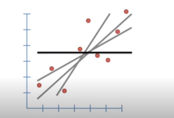
Stat Quest Stat QuestLet say the bold line (‘b’), represents the average Y value and distance between b and all the datapoints known as residual.
假设粗线('b')表示平均Y值以及b与所有称为残差的数据点之间的距离。
(b-Y1) is the distance between b and the first datapoint. Similarly, (b-y2) and (b-Y3) is the distance between second and third datapoints and so on.
(b-Y1)是b与第一个数据点之间的距离。 同样,(b-y2)和(b-Y3)是第二和第三数据点之间的距离,依此类推。
Note: Some of the datapoints are less than b and some are bigger so on adding they cancel out each other, therefore we take the squares of the sum of residuals.
注意 :有些数据点小于b,有些数据点较大,因此加起来它们会互相抵消,因此我们采用残差总和的平方。
SSR = (b-Y1)² + (b-Y2)² + (b-Y3)² + ………… + ……(b-Yn)² . where, n is the number of datapoints.
SSR =(b-Y1)²+(b-Y2)²+(b-Y3)²+…………+……(b-Yn)² 。 其中,n是数据点的数量。
When for the line SSR is very less, the line is considered to be the best fit line. To find this best fit lines we need the help of equation of straight lines:
当直线的SSR很小时,该直线被认为是最合适的直线。 为了找到最佳拟合线,我们需要直线方程的帮助:
Y = mX+c
Y = mX + c
Where, m is the slope and c is the intercept through y_axis. Value of ‘m’ and ‘c’ should be optimal for SSR to be less.
其中,m是斜率,c是通过y_axis的截距。 对于SSR,“ m”和“ c”的值应最佳。
SSR = ((mX1+c)-Y1)² + ((mX2+c)-Y2)² + ………. + …….
SSR =((mX1 + c)-Y1)²+((mX2 + c)-Y2)²+…………。 +……。
Where Y1, Y2, ……., Yn is the observed/actual value and,
其中Y1,Y2,.......,Yn是观测值/实际值,并且
(mX1+c), (mX2+c), ………. Are the value of line or the predicted value.
(mX1 + c),(mX2 + c),…………。 是线的值还是预测值。
Since we want the line that will give the smallest SSR, this method of finding the optimal value of ‘m’ and ‘c’ is called Least-Square.
由于我们要的是能够提供最小SSR的线,因此这种找到'm'和'c'最佳值的方法称为最小二乘 。
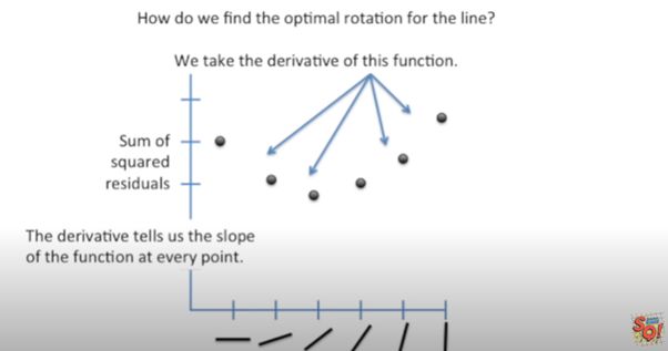
Stat Quest Stat QuestThis is the plot of SSR versus Rotation of Lines. SSR goes down when we start rotating the line, and after a saturation point it starts increasing on further rotation. The line of rotation for which SSR is minimal is the best fitted line. We can use derivation for finding this line. On derivation of SSR, we get the slope of the function at every point, when at the point the slope is zero, the model select that line.
这是SSR与线旋转的关系图。 当我们开始旋转线时,SSR会下降,并且在达到饱和点后,它会随着进一步旋转而开始增加。 SSR最小的旋转线是最佳拟合线。 我们可以使用推导找到这条线。 在推导SSR时,我们获得函数在每个点的斜率,当该点的斜率为零时,模型选择该线。
R-平方 (R-Squared)
R-Squared is the goodness-of-fit measure for the linear regression model. It tells us about the percentage of variance in the dependent variable explained by Independent variables. R-Squared measure strength of relationship between our model and dependent variable on 0 to 100% scale. It explains to what extent the variance of one variable explains the variance of second variable. If R-Squared of any model id 0.5, then half of the observed variation can be explained by the model’s inputs. R-Squared ranges from 0 to 1 or 0 to 100%. Higher the R², more the variation will be explained by the Independent variables.
R平方是线性回归模型的拟合优度度量。 它告诉我们有关自变量解释的因变量的方差百分比。 R平方测量模型与因变量之间的关系强度,范围为0至100%。 它解释了一个变量的方差在多大程度上解释了第二个变量的方差。 如果R-Squared的任何模型id为0.5,则可以通过模型的输入解释观察到的变化的一半。 R平方的范围是0到1或0到100%。 R²越高,自变量将解释更多的变化。
R² = Variance explained by model / Total variance
R²=用模型解释的方差/总方差
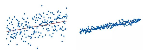
R² for the model on left is very less than that of the right.
左侧模型的R²远小于右侧模型的R²。
But it has its limitations:
但是它有其局限性:
· R² tells us the variance in dependent variable explained by Independent ones, but it does not tell whether the model is good or bad, nor will it tell you whether the data and predictions are biased. A high R² value doesn’t mean that model is good and low R² value doesn’t mean model is bad. Some fields of study have an inherently greater amount of unexplained variation. In these areas R² value is bound to be lower. E.g., study that tries to predict human behavior generally has lower R² value.
·R²告诉我们独立变量解释的因变量方差,但它不告诉模型好坏,也不会告诉您数据和预测是否有偏差。 高R²值并不表示模型良好,而低R²值并不意味着模型不好。 一些研究领域固有地存在大量无法解释的变化。 在这些区域中,R 2值必然较低。 例如,试图预测人类行为的研究通常具有较低的R²值。
· If we keep adding the Independent variables in our model, it tends to give more R² value, e.g., House cost prediction, number of doors and windows are the unnecessary variable that doesn’t contribute much in cost prediction but can increase the R² value. R Squared has no relation to express the effect of a bad or least significant independent variable on the regression. Thus, even if the model consists of a less significant variable say, for example, the person’s Name for predicting the Salary, the value of R squared will increase suggesting that the model is better. Multiple Linear Regression tempt us to add more variables and in return gives higher R² value and this cause to overfitting of model.
·如果我们继续在模型中添加自变量,那么它往往会提供更大的R²值,例如,房屋成本预测,门窗数量是不必要的变量,虽然对成本预测的贡献不大,但可以增加R²值。 R平方没有关系表示不良或最不重要的自变量对回归的影响。 因此,即使模型包含一个不太重要的变量,例如,用于预测薪水的人员姓名,R平方的值也会增加,表明该模型更好。 多元线性回归诱使我们添加更多变量,反过来又赋予了较高的R²值,这导致模型过度拟合。
Due, to its limitation we use Adjusted R-Squared or Predicted R-Squared.
由于其局限性,我们使用调整后的R平方或预测的R平方。
Calculation of R-Squared
R平方的计算
Project all the datapoints on Y-axis and calculate the mean value. Just like SSR, sum of squares of distance between each point on Y-axis and Y-mean is known as SS(mean).
将所有数据点投影到Y轴上并计算平均值。 与SSR一样,Y轴上每个点与Y均值之间的距离的平方和称为SS(mean)。
Note: (I am not trying to explain it as in mathematical formula, In Wikipedia and every other place the mathematical approach is given. But this is the theoretical way and the easiest way I understood it from Stat Quest. Before following mathematical approach, we should know the concept behind this).
注意 :(我不打算像维基百科中的数学公式那样解释它。 每隔一个地方都给出了数学方法。 但这是理论上的方法,也是我从Stat Quest了解它的最简单方法。 在遵循数学方法之前,我们应该了解其背后的概念)。
SS(mean) = (Y-data on y-axis — Y-mean)²
SS(平均值)=(y轴上的Y数据-Y平均值)²
SS(var) = SS(mean) / n .. where, n is number of datapoints.
SS(var)= SS(mean)/ n ..其中,n是数据点的数量。
Sum of Square around best fit line is known as SS(fit).
最佳拟合线周围的平方和称为SS(拟合)。
SS(fit) = (Y-data on X-axis — point on fit line)²
SS(fit)=(X轴上的Y数据-拟合线上的点)²
SS(fit) = (Y-actual — Y-predict)²
SS(fit)=(Y实际-Y预测)²
Var(fit) = SS(fit) / n
Var(拟合)= SS(拟合)/ n
R² = (Var(mean) — Var(fit)) / Var(mean)
R²=(Var(平均值)-Var(拟合))/ Var(平均值)
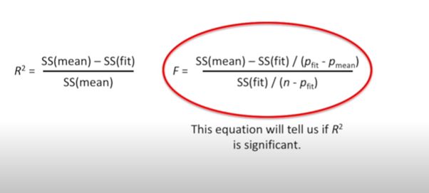
R² = (SS(mean) — SS(fit)) / SS(mean)
R²=(SS(平均值)-SS(拟合))/ SS(平均值)
R² = 1 — SS(fit)/SS(mean)
R²= 1-SS(拟合)/ SS(平均值)
Mathematical approach:
数学方法:
Here, SS(total) is same as SS(mean) i.e. SST (Total Sum of Squares) is the sum of the squares of the difference between the actual observed value y, and the average of the observed value (y mean) projected on y-axis.
在此,SS(total)与SS(mean)相同,即SST(总平方和)是实际观测值y与投影到实测值y的平均值之间的差的平方之和。 y轴。
Here, SSR is same as SS(fit) i.e. SSR (Sum of Squares of Residuals) is the sum of the squares of the difference between the actual observed value, y and the predicted value (y^).
在此,SSR与SS(fit)相同,即SSR(残差平方和)是实际观测值y与预测值(y ^)之差的平方和。
Adjusted R-Squared:
调整后的R平方:
Adjusted R-Squared adjusts the number of Independent variables in the model. Its value increases only when new term improves the model fit more than expected by chance alone. Its value decreases when the term doesn’t improve the model fit by sufficient amount. It requires the minimum number of data points or observations to generate a valid regression model.
调整后的R平方调整模型中自变量的数量。 仅当新术语使模型的拟合度超出偶然的预期时,其价值才会增加。 当该术语不能充分改善模型拟合时,其值会减小。 它需要最少数量的数据点或观测值才能生成有效的回归模型。
Adjusted R-Squared use Degrees of Freedom in its equation. In statistics, the degrees of freedom (DF) indicate the number of independent values that can vary in an analysis without breaking any constraints.
调整后的R平方使用自由度在其方程式中。 在统计数据中 ,自由度(DF)表示独立值的数量,这些独立值在分析中可以变化而不会破坏任何约束。
Suppose you have seven pair of shoes to wear each pair on each day without repeating. On Monday, you have 7 different choices of pair of shoes to wear, on Tuesday choices decreases to 6, therefore on Sunday you don’t have any choice to wear which shoes you gonna wear, you are stuck with only the last left one to wear. We have no freedom on Sunday. Therefore, degree of freedom is how much an independent variable can freely vary to analyse the parameters.
假设您每天要穿七双鞋,而不必重复。 在星期一,您有7种不同的鞋穿选择,在星期二,选择的鞋数减少到6,因此在星期天,您别无选择要穿哪双鞋,只穿了最后一双穿。 周日我们没有自由。 因此,自由度是自变量可以自由变化多少以分析参数。
Every time you add an independent variable to a model, the R-squared increases, even if the independent variable is insignificant. It never declines. Whereas Adjusted R-squared increases only when independent variable is significant and affects dependent variable. It penalizes you for adding independent variable that do not help in predicting the dependent variable.
每次向模型添加自变量时,即使自变量无关紧要, R平方 也会增加 。 它永远不会下降。 而仅当自变量显着且影响因变量时, 调整后R平方才会增加。 它会因添加无助于预测因变量的自变量而受到惩罚。
for detail understanding watch Krish Naik
了解更多细节,请观看 Krish Naik
P — Value
P —值
Suppose in a co-ordinate plane of 2-D, within the axis of x and y lies two datapoints irrespective of coordinates, i.e. anywhere in the plane. If we draw a line joining them it will be the best fit line. Again, if we change the coordinate position of those two points and again join them, then also that line will be the best fit. No matter where the datapoints lie, the line joining them will always be the best fit and the variance around them will be zero, that gives
假设在x和y轴内的2-D坐标平面中,存在两个数据点,而与坐标无关,即平面中的任何位置。 如果我们画一条线连接它们,那将是最合适的线。 同样,如果我们更改这两个点的坐标位置并再次连接它们,则该线也将是最合适的。 无论数据点位于何处,连接它们的线将始终是最佳拟合,并且它们周围的方差将为零,从而得出
value always 100%. But that doesn’t mean those two datapoints will always be statistically significant, i.e. always give the exact prediction of target variable. To know about the statistically significant independent variables that gives good R² value, we calculate P — value.
值始终为100%。 但这并不意味着这两个数据点在统计上始终是有意义的,即始终给出目标变量的准确预测。 要了解具有良好R²值的统计上显着的自变量,我们计算P —值。
Big Question — What is P — Value?
大问题-什么是P-值?
We still don’t know anything about P — Value. P — value is like Thanos and to defeat Thanos we have to deal with Infinity Stones first. P — value has its own infinity stones like alpha(α), F — score, z — score, Null Hypothesis, Hypothesis Testing, T-test, Z-test. Let’s first deal with F — score.
我们仍然对P —值一无所知。 P-价值就像Thanos并击败Thanos 我们必须先与Infinity Stones打交道。 P-值具有自己的无穷大石头,例如alpha(α),F-分数,z-分数,零假设,假设检验,T检验,Z检验。 首先处理F-分数。
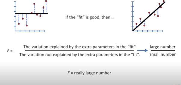
Stat Quest Stat Quest Stat Quest Stat QuestThe fit line is the variance explained by the extra parameters. The distance between the fit line and the actual datapoints is known as Residuals. These Residuals are the variation not explained by the extra parameters in the fit.
拟合线是额外参数解释的方差。 拟合线和实际数据点之间的距离称为残差。 这些残差是拟合中多余参数无法解释的变化。
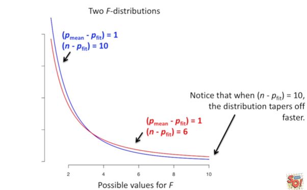
For different random sets of datapoints (or samples), there will be different calculated F. let say, for thousands of samples there will be thousands of F. If we plot all the F on histogram plot, it will look something like this.
对于不同的随机数据点集(或样本),将有不同的计算得出的F。可以说,对于成千上万的样本,将有成千上万的F。如果我们在直方图上绘制所有F,则看起来像这样。
If we draw a line connecting the outer of all the F, we get like this
如果我们画一条连接所有F外部的线,我们将得到这样的结果
The shape of the line is been determined by the degrees of freedom
线的形状由自由度确定
For the red line the sample size is smaller than the sample size of blue line, the blue line with more sample size is narrowing towards x-axis faster than that of red line. If the sample size is greater relative to the number of parameters in fit line then P — value will be smaller.
对于红线,样本大小小于蓝线的样本大小,具有更多样本大小的蓝线向x轴的收缩速度比红线快。 如果样本大小相对于拟合线中的参数数量更大,则P —值将更小。
For further clear understanding about P — value, we need to first understand about the Hypothesis Testing.
为了进一步清楚地了解P值,我们需要首先了解假设检验。
Hypothesis Testing –
假设检验 -
What is Hypothesis? Any guess done by us is Hypothesis. E.g.
假设是什么? 我们所做的任何猜测都是假设。 例如
1. On Sunday, Peter always play Basketball.
1.星期天,彼得总是打篮球。
2. A new vaccine for corona will work great.
2.一种新的电晕疫苗效果很好。
3. Sachin always scores 100 on Eden.
3.萨钦(Sachin)在伊甸园(Eden)总是得分100。
4. NASA may have detected a new species.
4. NASA可能检测到新物种。
5. I can have a dozen eggs at a time. Etc. etc.
5.我一次可以打十二个鸡蛋。 等等
If we put all the above guessed sentence on a test, it is known as Hypothesis Testing.
如果我们将以上所有猜测的句子放在测试中,则称为假设测试。
1. If tomorrow is Sunday, then Peter will be found playing Basketball.
1.如果明天是星期天,那么彼得将被发现打篮球。
2. If this is the vaccine made for corona then it will work on corona patient.
2.如果这是用于电晕的疫苗,那么它将对电晕患者有效。
3. If the match is going at Eden, then Sachin will score 100.
3.如果比赛在伊甸园进行,那么萨钦将获得100分。
4. If there is any new species came to Earth, then it would have been detected by NASA.
4.如果有任何新物种进入地球,那么它就会被NASA探测到。
5. If I had taken part in Egg eating competition, then I could have eaten a dozen egg at a time and might have won the competition.
5.如果我参加了吃鸡蛋比赛,那么我一次可以吃十几个鸡蛋,并可能赢得比赛。
6. If I regularly give water to plant, it will grow nice and strong.
6.如果我定期给植物浇水,它会长得好壮。
7. If I’ll have a good coffee in morning, then I’ll work all day without being tired. Etc. etc.
7.如果我早上可以喝杯咖啡,那么我会整天工作而不累。 等等
You make a guess (Hypothesis), put it to test (Hypothesis testing). According to the University of California, a good Hypothesis should include both “If” and “then” statement and should include independent variable and dependent variable and can be put to test.
您进行猜测(假设),然后进行检验(假设测试)。 根据加利福尼亚大学的说法,一个好的假设应同时包含“ If”和“ then”陈述,并应包含自变量和因变量,并可以进行检验。
Null Hypothesis –
零假设 -
Null Hypothesis is the guess that we made. Any known fact can be a Null Hypothesis. Every guess we made above is Null Hypothesis. It can also be, e.g. our solar system has eight planets (excluding Pluto), Buffalo milk has more fat than that of cow, a ball will drop more quickly than a feather if been dropped freely from same height in vacuum.
零假设 是我们所做的猜测。 任何已知的事实都可以是零假设。 我们上面所做的每一个猜测都是零假设。 也可能是这样的,例如我们的太阳系有八个行星(不包括冥王星),水牛乳的脂肪比牛的脂肪多,如果在真空中从相同高度自由掉落,则球掉落的速度将比羽毛快。
Now here’s a catch. We can accept the Null Hypothesis or can reject the Null Hypothesis. We perform test on Null Hypothesis based on same observation or data, if the Hypothesis is true then we accept it or else we reject it.
现在有一个陷阱。 我们可以接受零假设,也可以拒绝零假设。 我们基于相同的观察或数据对空假设进行检验,如果假设为真,则我们接受该假设,否则我们拒绝该假设。
Big Question? How this test is done?
大问题? 该测试如何完成?
We evaluate two mutual statement on a Population (millions of data containing Independent and dependent variables) data using sample data (randomly chosen small quantity of data from a big data). For testing any hypothesis, we have to follow few steps:
我们使用样本数据(从大数据中随机选择的少量数据)评估总体 ( 人口数据(包含自变量和因变量的数百万个数据))上的两个相互陈述。 为了检验任何假设,我们必须遵循几个步骤:
1. Make an assumption.
1.做一个假设。
For e.g. let say A principal at a certain school claims that the students in his school are above average intelligence. A random sample of thirty students IQ scores have a mean score of 112. Is there sufficient evidence to support the principal’s claim? The mean population IQ is 100 with a standard deviation of 15.
例如,假设某所学校的一位校长声称他所在学校的学生的智力高于平均水平。 随机抽取 30名学生的智商得分, 平均得分为112。是否有足够的证据支持校长的主张? 总体智商平均为100, 标准差为15。
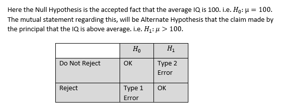
Here the Null Hypothesis is the accepted fact that the average IQ is 100. i.e.
在这里,零假设是公认的事实,即平均智商为100。即
Let say that after testing our Null Hypothesis is true, i.e. the claim made by principal that average IQ of students is above 100 is wrong. We chosen different sets of 30 students and took their IQ and averaged it and found in most cases that the average IQ is not more than 100. Therefore, our Null Hypothesis is true and we reject Alternate Hypothesis. But let say that due to lack of evidence we can’t able to find out the result or somehow mistakenly (two or three students are exceptionally brilliant with much more IQ) we calculated that average IQ is above 100 but the actual correct result is average IQ is 100 and we reject Null Hypothesis, this is Type 1 error.
可以说,在检验了我们的零假设之后,就是正确的,也就是说,校长声称学生的平均智商高于100是错误的。 我们选择了30个学生的不同集合,并对其智商进行平均,发现在大多数情况下,平均智商不超过100。因此,我们的零假设是真实的,而我们拒绝替代假设。 但是可以说,由于缺乏证据,我们无法找到结果或以某种方式错误地发现(两到三名学生非常聪明,智商更高),我们计算出平均智商高于100,但实际正确结果是平均IQ为100,我们拒绝空假设,这是1类错误。
Again, let say that the Null Hypothesis is true, average IQ of students is not more than 100. But due to presence of those exceptionally brilliant students we got the average IQ above 100, so we do not reject Alternate Hypothesis. That is type 2 error.
再次,让我们假设“零假设”是正确的,学生的平均智商不超过100。但是,由于这些出色的学生的存在,我们使平均智商高于100,因此我们不会拒绝“替代假设”。 那是类型2错误。
It’s confusing though. Okay let’s take another example.
不过这很令人困惑。 好吧,让我们再举一个例子。
Suppose a person is somehow convicted but he is innocent, he just accidentally found present near a dead body and got convicted. Here Null Hypothesis, is person is innocent. Alternate Hypothesis can be that person is guilty but due to lack of evidence, person got charged and punished by law. So, it is Type 1 error. But what if person is actually guilty. He claimed that he is innocent, Alternate hypothesis suggested he is guilty but due to lack of evidence, he got bailed and charged free. This is type 2 error (not rejecting Alternate Hypothesis).
假设某人被定罪,但他是无辜的,他只是偶然发现尸体附近存在并被定罪。 在这里零假设,就是人无辜。 替代假设可能是某人有罪,但由于缺乏证据,该人被起诉并受到法律制裁。 因此,这是Type 1错误。 但是如果人确实有罪怎么办。 他声称自己是无辜的,另一种假设表明他有罪,但由于缺乏证据,他获得了保释并被释放。 这是2类错误(不拒绝替代假设)。
- Choose the alpha(α), α is the significance level which is probability of making wrong decision when Null Hypothesis is true, i.e. probability of making type 1 error. Generally, we choose α = 0.05, it’s okay if for less than 5 % of cases Null Hypothesis is proven wrong, we still consider it. But if Null hypothesis is wrong more than in 5% case then we reject it and accept Alternate Hypothesis. For important decision, like in medical cases or share market we do not take α > 0.03, it could be risk even if we avoid a minute error in these cases. 选择alpha(α),α是显着性水平,当无效假设为真时,它是做出错误决策的概率,即发生类型1错误的概率。 通常,我们选择α= 0.05,如果在不到5%的情况下,零假设被证明是错误的,我们仍然会考虑,那就可以了。 但是,如果空假设的错误率超过5%,则我们将其拒绝并接受替代假说。 对于重要决策,例如在医疗案例或股票市场中,我们不使α> 0.03,即使在这些案例中避免了微小的误差,也可能存在风险。
- 1. Perform the test. 1.执行测试。
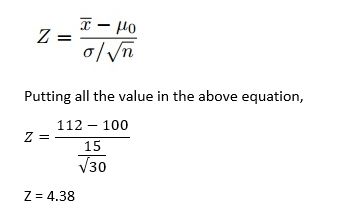
Z— test
Z—检验
Here, X(bar) is the sample mean, i.e. Average IQ of randomly chosen 30 students which is 112.
这里的X(bar)是样本平均值,即随机选择的30名学生的平均智商为112。
(Mu-0) is the population mean, i.e. Average IQ of all students that is 100.
(Mu-0)是人口平均值,即所有学生的平均智商为100。
(sigma) is the standard deviation, i.e. how much data is varying from the population mean?
(sigma)是标准偏差,即,与总体平均值相比有多少数据不同?
n is the sample size that is 30.
n是30的样本量。
Let’s discuss about the Normal distribution and Z-score before performing the test.
在执行测试之前,让我们讨论正态分布和Z分数。
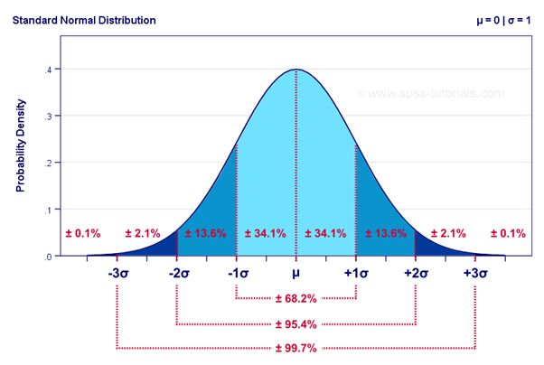
Normal Distribution
正态分布
Properties:
特性:
· Bell shaped curve
·钟形曲线
· No skewness
·无偏斜
· Symmetrical
·对称
· In normal distribution,
·在正态分布中,
Mean = median = mode
平均值=中位数=模式
Area Under Curve is 100% or 1
曲线下面积为100%或1
Mean = 0 and standard deviation, σ = 1
均值= 0和标准偏差σ= 1
Z — score
Z-得分
Z — score tells us that how much a data, a score, a sample is been deviated from the mean of normal distribution. By the help of Z — score we can convert any score or sample distribution with mean and standard deviation other than that of a normal distribution, (i.e. when the data is skewed) to the mean and deviation of normal distribution of mean equal to zero and deviation equal to one.
Z-得分 告诉我们,数据,得分,样本有多少偏离了正态分布的均值。 借助Z-评分,我们可以将除正态分布外的均值和标准差(即,当数据偏斜时)的任何得分或样本分布转换为均值和均值的正态分布与均值的偏差,均值等于零,偏差等于一。
From Z — score table, an area of α = 0.05 is equal to 1.645 of Z — score, which is smaller than Z value we get. So we will reject the Null Hypothesis in this case.
从Z_分数表中 , α= 0.05的面积等于Z_分数的1.645,小于我们得到的Z值。 因此,在这种情况下,我们将拒绝零假设。
Now, we got the Z — score, we can calculate P — value, by the help of Normal Distribution Table:
现在,我们得到了在Z -得分,我们可以计算出P -值 ,通过帮助正态分布表:
By looking at Normal Distribution table we get that Z — value for the value less than — 3 is 0.001. If the P — value < 0.05, we reject the Null Hypothesis.
通过查看正态分布表,我们得出Z值小于-3的值为0.001。 如果P值<0.05,则我们拒绝零假设。
Big.. Big Confusion –
大..大混乱–
We often tend to confuse between probability and P — value. But there is a big difference between them. Let’s take an example.
我们常常倾向于混淆概率和P值。 但是它们之间有很大的区别。 让我们举个例子。
By flipping a coin, we can get the chance of coming of head is 50%. If we flip another coin, again the chance of getting a head is 50%.
通过掷硬币,我们可以获得正面的机会是50%。 如果我们掷另一枚硬币,再次获得正面的机会是50%。
Now, what’s the probability of getting two head in a row and what’s the P — value of getting two head in a row?
现在,连续获得两个头的概率是多少?连续获得两个头的P值是多少?
On flipping of two coins simultaneously,
同时翻转两枚硬币时,
Total outcome = HH, HT, TH, TT = 4
总结果= HH,HT,TH,TT = 4
Favorable outcome = HH = 1
有利的结果= HH = 1
P(HH) = ¼ = 0.25, and P(TT) = ¼ = 0.25
P(HH)=¼= 0.25,P(TT)=¼= 0.25
P(one H or one T) =(HT,TH)/(HH,HT,TH,TT)=2/4=0.5
P(一个H或一个T)=(HT,TH)/(HH,HT,TH,TT)= 2/4 = 0.5
P — value is the probability that the random chance generated the data, or something else that is equal or rarer.
P —值是随机机会生成数据的概率,或者等于或稀少的其他概率。
Therefore, probability of getting two heads in a row is 0.25 and P — value for getting two heads in a row is 0.5.
因此,连续获得两个头的概率为0.25,连续获得两个头的P_值为0.5。
All the graphical plots are taken from Stat Quest. for this article I have followed Stat Quest and Krish Naik.
所有图形图均取自Stat Quest。 对于本文,我关注了Stat Quest和Krish Naik 。
If something is missing here or explained wronged, then please comment and guide me through it.
如果此处缺少或解释有误,请发表评论并指导我。
翻译自: https://medium.com/@asitdubey.001/linear-regression-and-fitting-a-line-to-a-data-6dfd027a0fe2
