SCS【8】单细胞转录组之筛选标记基因 (Monocle 3)

点击关注，桓峰基因

Topic 6. 克隆进化之 Canopy

Topic 7. 克隆进化之 Cardelino

Topic 8. 克隆进化之 RobustClone

SCS【1】今天开启单细胞之旅，述说单细胞测序的前世今生

SCS【2】单细胞转录组 之 cellranger

SCS【3】单细胞转录组数据 GEO 下载及读取

SCS【4】单细胞转录组数据可视化分析 (Seurat 4.0)

SCS【5】单细胞转录组数据可视化分析 (scater)

SCS【6】单细胞转录组之细胞类型自动注释 (SingleR)

SCS【7】单细胞转录组之轨迹分析 (Monocle 3) 聚类、分类和计数细胞

SCS【8】单细胞转录组之筛选标记基因 (Monocle 3)

---

这期继续介绍 Monocle 3 软件包用于筛选每个cluster的标记基因。

前言

单细胞转录组测序(scRNA-seq)实验使我们能够发现新的细胞类型，并帮助我们了解它们是如何在发育过程中产生的。Monocle 3包提供了一个分析单细胞基因表达实验的工具包。

Monocle 3可以执行三种主要类型的分析:

1. 聚类、分类和计数细胞。单细胞RNA-Seq实验允许发现新的(可能是罕见的)细胞亚型。

2. 构建单细胞轨迹。在发育、疾病和整个生命过程中，细胞从一种状态过渡到另一种状态。Monocle 3可以发现这些转变。

3. 差异表达分析。对新细胞类型和状态的描述，首先要与其他更容易理解的细胞进行比较。Monocle 3包括一个复杂的，但易于使用的表达系统。

工作流程图如下：

也就是流程图中的黄色框框的部分，包括筛选每个 cluster 中的标记基因，并对此进行细胞的注释。

软件包安装

软件包除了需要我们安装Monocle 3之外，还需要安装 garnett 用于细胞注释的软件包，安装如下：

if (!requireNamespace("BiocManager", quietly = TRUE))
  install.packages("BiocManager")
  BiocManager::install(version = "3.14")
  
BiocManager::install(c('BiocGenerics', 'DelayedArray', 'DelayedMatrixStats',
                       'limma', 'lme4', 'S4Vectors', 'SingleCellExperiment',
                       'SummarizedExperiment', 'batchelor', 'Matrix.utils',
                       'HDF5Array', 'terra', 'ggrastr'))

install.packages("devtools")
devtools::install_github('cole-trapnell-lab/monocle3')
## Install the monocle3 branch of garnett
BiocManager::install(c("org.Mm.eg.db", "org.Hs.eg.db"))
devtools::install_github("cole-trapnell-lab/garnett", ref="monocle3")

# install gene database for worm
BiocManager::install("org.Ce.eg.db")

数据读取

数据读取我们可以参考上期 SCS【7】单细胞转录组之轨迹分析 (Monocle 3) 聚类、分类和计数细胞 。这里数据读取也完整的给出来，我们对数据分析到第四步利用 UMAP对数据进行降维聚类，当然有需要也可以选择 t-SNE 方法，如下：

library(monocle3)
expression_matrix <- readRDS("cao_l2_expression.rds")
cell_metadata <- readRDS("cao_l2_colData.rds")
gene_annotation <- readRDS("cao_l2_rowData.rds")


# Make the CDS object
cds <- new_cell_data_set(expression_matrix, cell_metadata = cell_metadata, gene_metadata = gene_annotation)
cds
## Step 1: Normalize and pre-process the data
cds <- preprocess_cds(cds, num_dim = 100, method = c("PCA", "LSI"))
plot_pc_variance_explained(cds)

## Step 2: Remove batch effects with cell alignment cds <- align_cds(cds,
## alignment_group = 'batch')

## Step 3: Reduce the dimensions using 'UMAP', 'tSNE', 'PCA', 'LSI', 'Aligned'
cds <- reduce_dimension(cds, reduction_method = "UMAP")

## Step 4: Cluster the cells
cds <- cluster_cells(cds)
plot_cells(cds)

例子实操

一旦细胞聚集起来，我们就想知道是什么基因使它们彼此不同。要做到这一点，首先调用 top_markers()函数，数据框 marker_test_res 包含了许多关于每个分区中每个基因的具体表达方式的度量。我们可以根据 cluster 、partition 或 colData(cds) 中的任何变量对细胞进行分组。您可以根据一个或多个特异性指标对其进行排序，并选取每个聚类取最上面的基因。例如，pseudo_R2 就是这样一个度量。我们可以根据 pseudo_R2 对 markers 进行排序，如下所示:

筛选标记基因

library(dplyr)
marker_test_res <- top_markers(cds, group_cells_by = "partition", reference_cells = 1000,
    cores = 8)
top_specific_markers <- marker_test_res %>%
    filter(fraction_expressing >= 0.1) %>%
    group_by(cell_group) %>%
    top_n(1, pseudo_R2)

top_specific_marker_ids <- unique(top_specific_markers %>%
    pull(gene_id))

我们可以用 plot_genes_by_group 函数绘制每组中表达每种 markers 的细胞的表达和比例:

plot_genes_by_group(cds, top_specific_marker_ids, group_cells_by = "partition", ordering_type = "maximal_on_diag",
    max.size = 3)

查看多个 markers 通常会提供更多信息，你可以通过将top_n()的第一个参数改为 3 来实现:

####### top_n(3)##
top_specific_markers <- marker_test_res %>%
    filter(fraction_expressing >= 0.1) %>%
    group_by(cell_group) %>%
    top_n(3, pseudo_R2)

top_specific_marker_ids <- unique(top_specific_markers %>%
    pull(gene_id))

plot_genes_by_group(cds, top_specific_marker_ids, group_cells_by = "partition", ordering_type = "cluster_row_col",
    max.size = 3)

细胞类型注释

识别数据集中每个细胞的类型对于许多下游分析是至关重要的。有几种方法可以做到这一点。一种常用的方法是首先将细胞聚类，然后根据其基因表达谱为每一簇分配一种细胞类型。

1. 根据类型注释细胞

我们已经看到了如何使用top_markers()。回顾与标记基因相关的文献，通常会给出表达该基因的簇的身份的强烈指示。在Cao & Packer >等人的研究中，作者查阅了文献和基因表达数据库中限制在每个聚类的标记，以便分配colData(cds)$cao_cell_type中包含的身份。

要基于cluster分配细胞类型，我们首先在colData(cds)中创建一个新列，并用 partitions(cds) 的值初始化它(也可以使用clusters(cds)，这取决于你的数据集):

colData(cds)$assigned_cell_type <- as.character(partitions(cds))
colData(cds)$assigned_cell_type <- dplyr::recode(colData(cds)$assigned_cell_type,
    `1` = "Body wall muscle", `2` = "Germline", `3` = "Motor neurons", `4` = "Seam cells",
    `5` = "Sex myoblasts", `6` = "Socket cells", `7` = "Marginal_cell", `8` = "Coelomocyte",
    `9` = "Am/PH sheath cells", `10` = "Ciliated neurons", `11` = "Intestinal/rectal muscle",
    `12` = "Excretory gland", `13` = "Chemosensory neurons", `14` = "Interneurons",
    `15` = "Unclassified eurons", `16` = "Ciliated neurons", `17` = "Pharyngeal gland cells",
    `18` = "Unclassified neurons", `19` = "Chemosensory neurons", `20` = "Ciliated neurons",
    `21` = "Ciliated neurons", `22` = "Inner labial neuron", `23` = "Ciliated neurons",
    `24` = "Ciliated neurons", `25` = "Ciliated neurons", `26` = "Hypodermal cells",
    `27` = "Mesodermal cells", `28` = "Motor neurons", `29` = "Pharyngeal gland cells",
    `30` = "Ciliated neurons", `31` = "Excretory cells", `32` = "Amphid neuron",
    `33` = "Pharyngeal muscle")

plot_cells(cds, group_cells_by = "partition", color_cells_by = "assigned_cell_type")

Partition 7 有一些子结构，仅从top_markers()的输出中看不出它对应的单元格类型是什么。所以我们可以用choose_cells()函数将它分离出来以便进一步分析:

cds_subset <- choose_cells(cds)

现在我们有了一个更小的cell_data_set对象，只包含我们想要筛选的细胞。我们可以使用 graph_test() 来识别在该分区的不同细胞子集中差异表达的基因:

pr_graph_test_res <- graph_test(cds_subset, neighbor_graph = "knn", cores = 8)
pr_deg_ids <- row.names(subset(pr_graph_test_res, morans_I > 0.01 & q_value < 0.05))
gene_module_df <- find_gene_modules(cds_subset[pr_deg_ids, ], resolution = 0.001)
plot_cells(cds_subset, genes = gene_module_df, show_trajectory_graph = FALSE, label_cell_groups = FALSE)

也可以探索每个模块中的基因，或对它们进行 GO 富集分析，以收集关于存在哪些细胞类型的解读。假设做完这些之后，我们对分区中的细胞类型有了很好的了解。让我们以更好的分辨率重新聚类的细胞，然后看看它们是如何与分区中聚类重叠的:

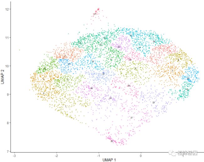
cds_subset <- cluster_cells(cds_subset, resolution = 0.01)
plot_cells(cds_subset, color_cells_by = "cluster")

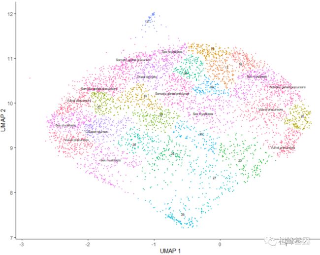
基于模式的排列方式，我们将进行以下分配:

colData(cds_subset)$assigned_cell_type <- as.character(clusters(cds_subset)[colnames(cds_subset)])
colData(cds_subset)$assigned_cell_type <- dplyr::recode(colData(cds_subset)$assigned_cell_type,
    `1` = "Sex myoblasts", `2` = "Somatic gonad precursors", `3` = "Vulval precursors",
    `4` = "Sex myoblasts", `5` = "Vulval precursors", `6` = "Somatic gonad precursors",
    `7` = "Sex myoblasts", `8` = "Sex myoblasts", `9` = "Ciliated neurons", `10` = "Vulval precursors",
    `11` = "Somatic gonad precursor", `12` = "Distal tip cells", `13` = "Somatic gonad precursor",
    `14` = "Sex myoblasts", `15` = "Vulval precursors")

plot_cells(cds_subset, group_cells_by = "cluster", color_cells_by = "assigned_cell_type")

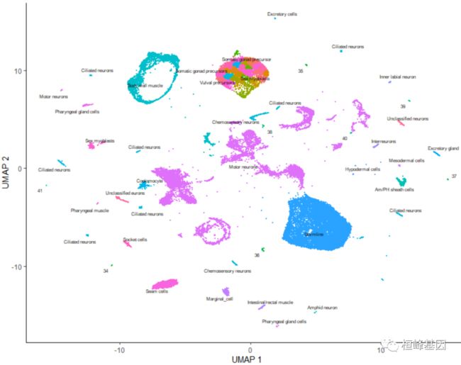
现在，我们可以将 cds_subset 对象中的注释传输回完整的数据集。在这个阶段，我们还会过滤掉低质量的细胞：

colData(cds)[colnames(cds_subset), ]$assigned_cell_type <- colData(cds_subset)$assigned_cell_type
cds <- cds[, colData(cds)$assigned_cell_type != "Failed QC" | is.na(colData(cds)$assigned_cell_type)]
plot_cells(cds, group_cells_by = "partition", color_cells_by = "assigned_cell_type",
    labels_per_group = 5)

2. Automated annotation with Garnett

上面按类型手动注释单元格的过程可能很费力，如果底层聚类发生变化，则必须重新执行。最近开发了Garnett，这是一个自动注释细胞的软件工具包。Garnett 根据标记基因对细胞进行分类。如果您已经经历了手工注释细胞的麻烦，Monocle可以生成一个标记基因文件，可以与 Garnett 一起使用。这将帮助您在将来注释其他数据集，或者在将来改进分析和更新聚类时重新注释这个数据集。

要生成一个Garnett文件，首先找到每个带注释的细胞类型所表示的顶部标记:

## Automated annotation with Garnett
assigned_type_marker_test_res <- top_markers(cds, group_cells_by = "assigned_cell_type",
    reference_cells = 1000, cores = 8)
# Require that markers have at least JS specificty score > 0.5 and be
# significant in the logistic test for identifying their cell type:
garnett_markers <- assigned_type_marker_test_res %>%
    filter(marker_test_q_value < 0.01 & specificity >= 0.5) %>%
    group_by(cell_group) %>%
    top_n(5, marker_score)
# Exclude genes that are good markers for more than one cell type:
garnett_markers <- garnett_markers %>%
    group_by(gene_short_name) %>%
    filter(n() == 1)

head(garnett_markers)
generate_garnett_marker_file(garnett_markers, file = "./marker_file.txt")

最终将生成如下的文本文件:

> Cell type 35
expressed: abf-2, Y45F3A.8, Y62F5A.9, F48E3.8, R05G6.9

> Cell type 36
expressed: col-12, col-89, col-130, col-159, col-167

> Cell type 40
expressed: col-14, col-97, col-113, R07B1.8, grl-6

> Cell type Body wall muscle
expressed: col-107, iff-1, plk-3, ram-2, T19H12.2

> Cell type Germline
expressed: csq-1, icl-1, F37H8.5, hum-9, F41C3.5

> Cell type Seam cells
expressed: cup-4, inos-1, Y73F4A.1, ZC116.3, aman-1

现在根据你的标记文件像这样训练一个 Garnett 分类器，现在我们已经训练了一个分类器 worm_classifier，我们可以使用它来根据类型注释 L2 细胞，以下是 Garnett 对这些细胞的注释过程：

library(garnett)
worm_classifier <- train_cell_classifier(cds = cds, marker_file = "./marker_file.txt",
    db = org.Ce.eg.db::org.Ce.eg.db, cds_gene_id_type = "ENSEMBL", num_unknown = 50,
    marker_file_gene_id_type = "SYMBOL", cores = 8)
cds <- classify_cells(cds, worm_classifier, db = org.Ce.eg.db::org.Ce.eg.db, cluster_extend = TRUE,
    cds_gene_id_type = "ENSEMBL")
plot_cells(cds, group_cells_by = "partition", color_cells_by = "cluster_ext_type")

我们这期先分析第一部分，内容过多，一次完成有点太乱了，目前单细胞测序的费用也在降低，单细胞系列可算是目前的测序神器，有这方面需求的老师，联系桓峰基因，提供最高端的科研服务！

桓峰基因，铸造成功的您！

未来桓峰基因公众号将不间断的推出单细胞系列生信分析教程，

敬请期待！！

有想进生信交流群的老师可以扫最后一个二维码加微信，备注“单位+姓名+目的”，有些想发广告的就免打扰吧，还得费力气把你踢出去！

References:

1. G. X. Y. Zheng, et al, Massively parallel digital transcriptional profiling of single cells. Nat. Commun. 8, 14049 (2017). doi:10.1038/ncomms14049pmid:28091601