异常行为检测算法
Anomaly detection is a critical problem that has been researched within diverse research areas and application disciplines. This article aims to construct a structured and comprehensive overview of the selected algorithms for anomaly detection by targeting data scientists, data analysts, and machine learning specialists as an audience.
异常检测是已在各种研究领域和应用学科中研究的一个关键问题。 本文旨在通过将数据科学家,数据分析师和机器学习专家作为受众,针对所选的异常检测算法构建结构全面的概述。
异常检测的概念 (Concept of Anomaly Detection)
An unexpected change that performs highly divergent attitudes from other observations in a time period can be represented as abnormal behavior. In other words, Anomaly Detection can be defined as the measure of specifying the outliers in the existing dataset which acts considerably different from the rest of the data points by profiling them as non-conforming normal points.
在一段时间内与其他观察结果表现出高度分歧的意外变化可以表示为异常行为。 换句话说,异常检测 可以定义为在现有数据集中指定离群值的度量,该离群通过将它们配置为不合格的法线点而与其余数据点有很大不同。
Anomalous points might be produced by errors in the data; however, it could point out to a historically or currently existing unidentified or hidden process or behavior by Hawkins.
异常点可能是由数据错误产生的; 但是,它可能指出了Hawkins在历史上或当前存在的未识别或隐藏的过程或行为。
As the publicly available data volume reaches in mass amounts, outlier detecting algorithms are modified to run on these data sets to be able to predict the unusual patterns. For instance, a “suspiciously high” count of login trials might outline a possible cyber intrusion or a considerable increase in incoming network traffic can be pointed to malicious activity in network systems. Considering these activities, they hold a shared aspect that they are “appealing” and “unusual” to the data scientists and data analysts. The “curiosity” or real-life applicability of anomalies is an essential element of anomaly detection.
随着公开可用数据量的大量增加,离群值检测算法已修改为在这些数据集上运行,以便能够预测异常模式。 例如,登录试验的“可疑数量”可能概述了可能的网络入侵,或者传入网络流量的显着增加可能表明网络系统中存在恶意活动。 考虑到这些活动,它们具有一个共同的方面,即它们对数据科学家和数据分析师“具有吸引力”和“不同寻常” 。 异常的“好奇心”或现实适用性是异常检测的基本要素。
异常类型 (Types of Anomalies)
There exist three different kinds of anomalies in the literature.
文献中存在三种不同类型的异常。
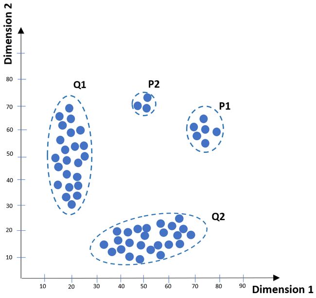
Figure 1. Types & Examples of Anomaly Detection. (Image by the author) 图1.异常检测的类型和示例。 (图片由作者提供)Descriptions can be found below:
可以在下面找到说明:
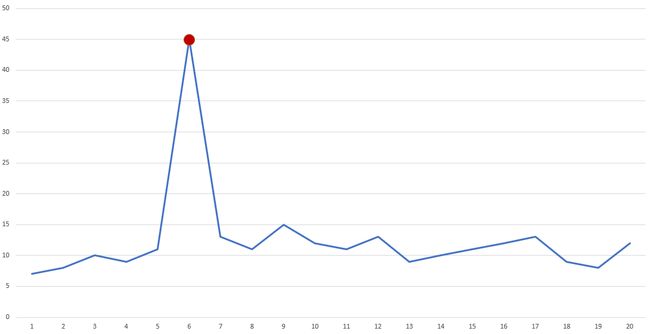
1. Point Anomaly: An anomaly when a distinct item in a dataset is largely dissimilar from others corresponding to its attributes.
1.点异常:数据集中的不同项目与对应于其属性的其他项目在很大程度上不同时的异常。
Figure 2. The point anomaly is marked with red. (Image by the author) 图2.点异常标记为红色。 (图片由作者提供)2. Contextual Anomalies: An anomaly which has a divergence that points to a context-based knowledge. This kind of anomaly may not be recognized when the contextual information is absent.
2.上下文异常:具有差异的异常,该异常指向基于上下文的知识。 当缺少上下文信息时,可能无法识别这种异常。
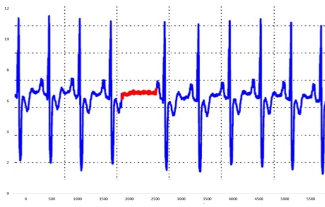
Figure 3. The contextual anomalous point that can be explained in its context. (Image by Author) 图3.可以在上下文中解释的上下文异常点。 (图片由作者提供)3. Collective Anomalies: Anomalies that are composed of multiple related instances of elements that may not constitute an anomalous point individually. The collective summation of specific events is considered while analyzing outlier behaviors.
3.集体异常:由元素的多个相关实例组成的异常,这些元素可能不会单独构成异常点。 在分析异常行为时,应考虑特定事件的集体汇总。
Figure 4. Collective Anomaly Detection highlighted in the red line. (Image by the author) 图4.红线中突出显示的集体异常检测。 (图片由作者提供)目录 (Table of Contents)
1. Statistical Approach1.1. Minimum Covariance Determinant (MCD)1.2. Principle Component Analysis (PCA)
1.统计方法1.1。 最小协方差决定因素(MCD) 1.2。 主成分分析(PCA)
2. Distance-based Approach
2.1. Local Outlier Factor (LOF)
2.2. Novelty Detection Local Outlier Factor (ND LOF)
2.3. Mahalanobis Distance (MDist)2.基于距离的方法2.1。 局部离群因子(LOF) 2.2。 新奇检测局部离群因子(ND LOF) 2.3。 马氏距离(MDist)
3. Density-based Approach
3.1. Density-Based Spatial Clustering of Applications with Noise (DBSCAN)
3.2. Ordering Points To Identify the Clustering Structure (OPTICS)3.基于密度的方法3.1。 基于密度的噪声应用空间聚类(DBSCAN) 3.2。 识别聚类结构的排序点(OPTICS)
4. Isolation-based Approach
4.1. Isolation Forest (iForest)4.基于隔离的方法4.1。 隔离林(iForest)
5. Classification-based Approach
5.1. One-Class SVM5.基于分类的方法5.1。 一类SVM
1.统计方法 (1. STATISTICAL APPROACH)
1.1。 最小协方差行列式(MCD) (1.1. Minimum Covariance Determinant (MCD))
Minimum Covariance Determinant (MCD) acts as the covariance estimator that is to be applied to Gaussian-distributed data. It basically searches for the subset of a specified number of data points whose covariance matrix contains the lowest determinant.
最小协方差行列式(MCD) 用作将应用于高斯分布数据的协方差估计器。 它基本上搜索指定数量的数据点的子集,这些数据点的协方差矩阵包含最低的行列式。
Because of the geometrical representation of the covariance matrix, the MCD algorithm tends to learn a rotationally symmetrical shape and works best with elliptically symmetric unimodal distributions. For this reason, it would be more performant to apply this algorithm while detecting outliers on the dataset which belongs to a unimodal distribution, so it is not advised to be used with multi-modal data. The more the size of the data and unimodality gets lower, the more the performance of the algorithm diminishes.
由于协方差矩阵的几何表示,MCD算法倾向于学习旋转对称的形状,并且最适合椭圆对称的单峰分布。 因此,在检测属于单峰分布的数据集上的离群值时,应用该算法会更有性能,因此不建议与多峰数据一起使用。 数据的大小和单峰性越小,算法的性能下降的幅度就越大。
For the formulation and the detailed parameter explanations, please kindly visit this article.
有关配方和详细的参数说明,请访问 这篇文章。
Figure 5. Classical Covariance Matrix (red) vs MCD Matrix (blue). (Image by the author) 图5.经典协方差矩阵(红色)与MCD矩阵(蓝色)。 (图片由作者提供)用于实现的Python库: (Python Library for Implementation:)
sklearn.covariance.MinCovDet
sklearn.covariance.MinCovDet
算法: (Algorithm:)
H: random subsample from X,
    [(I + J + 1) / 2 <= H <= I]

By using XH, the column-wise row vector mean can be computed as µH
For the covariance:: SH = (XH.T * XH) * (H -1)^(-1)The determinant of SH can be computed.
The squared Mahalanobis Distance for each observation in X as
    mi = (xi - µH)*SH^(-1) * (xi - µH).TAfter the computations, XH can be assigned as the subset of H observations with the smallest Mahalanobis Distance.
1.2。 主成分分析(PCA) (1.2. Principal Component Analysis (PCA))
This statistical methodology builds up the essentials of multivariate data analysis that uses an orthogonal transformation to apply on a set of observations of probably correlated variables into a set of values of uncorrelated variables in a linear way. It serves a multivariate table as a smaller set of variables to be able to inspect trends, bounces, and outliers. This type of high-level analysis may expose the interconnection between observations and variables.
这种统计方法建立了多元数据分析的基础 它使用正交变换以线性方式将一组可能的相关变量的观测值应用于一组不相关变量的值。 它将多变量表用作较小的变量集,以便能够检查趋势,反弹和离群值。 这种类型的高级分析可能会暴露观测值和变量之间的相互联系。
As one of the statistical anomaly detection approaches, it can be applied to, for instance, mark fraudulent transactions by evaluating applicable features to define what establishes as normal observation and assigning distance metrics to detect possible cases that serve as outliers/anomalies. This kind of approach allows training a model using the present unbalanced dataset.
作为统计异常检测方法之一,它可以通过评估适用的功能以定义确定为正常观察值的特征并分配距离度量以检测可能用作异常值/异常的情况,例如将其标记为欺诈性交易。 这种方法允许使用当前的不平衡数据集训练模型。
Figure 6. 2D PCA plot of clusters. (Image by the author) 图6.群集的2D PCA图。 (图片由作者提供)用于实现的Python库: (Python Library for Implementation:)
sklearn.decomposition.PCA
斯克莱恩分解
算法:(Algorithm:)
X = N × m    # Sample Covariance Matrixfor each data point xi
   X = subtract mean x from each column vector xi in X
   Σ = (X*X).T
return { λi, ui }i=(1..k)* Top-k vectors are more crucial eigenvectors
2.基于密度的方法 (2. DENSITY-BASED APPROACHES)
2.1。 基于密度的噪声应用空间聚类(DBSCAN) (2.1. Density-Based Spatial Clustering of Applications with Noise (DBSCAN))
The Density-Based Spatial Clustering of Applications with Noise (DBSCAN) aims to detect anomalous data points with the help of the density of its encircled space that is detached by regions of low-density observations.
带有噪声的应用程序的基于密度的空间聚类(DBSCAN) 旨在借助低密度观测区域所分离的环绕空间密度来检测异常数据点。
Major concepts of this methodology can be listed as density and connectivity which are calculated in terms of local distribution of their nearest neighbors.
该方法的主要概念可以列为密度和连通性,它们是根据其最近邻居的本地分布来计算的。
There exists two key parameters of the algorithm are:
该算法存在两个关键参数:
distance threshold — epsilon (ɛ): The given radius of the neighborhoods around a data point
距离阈值— epsilon(ɛ):数据点附近的给定半径
min_samples: The minimum number of data points in a neighborhood to create a cluster
min_samples:邻域中创建集群的最小数据点数
With the help of these parameters, the algorithm can be broken down in the following steps:
借助这些参数,可以按以下步骤分解算法:
Detecting the points in the ε (eps neighborhood of every point and identify the core points with more than minimum points neighbors.
在每个点的ε (eps邻域)中检测点,并标识与多个最小点相邻的核心点。
Find the connected components of inlier points on the neighbor graph, ignoring all non-core points.
忽略所有非核心点,在邻居图上找到内部点的连接分量。
Assign each non-inlier point to a nearby cluster if the cluster is an ε (eps neighbor, otherwise assign it to noise.
如果群集是ε(eps邻居),则将每个非内部点分配给附近的群集,否则将其分配给噪声。
A naive implementation of this requires storing the neighborhoods in step 1, thus requiring substantial memory. The original DBSCAN algorithm does not require this by performing these steps for one point at a time.
幼稚的实现需要在步骤1中存储邻域,因此需要大量内存。 原始DBSCAN算法不需要一次只执行一次这些步骤。
There are two parameters in the DBSCAN algorithm:
DBSCAN算法中有两个参数:
ε (epsilon): A point p is a core point if it has neighbors within a given radius
ε(ε):如果点p在给定半径内具有相邻点,则它是核心点
MinPts (minimum number of points): The least number of neighbors to form a cluster
最小点数 (最小点数):形成簇的最少邻居数
用于实现的Python库:(Python Library for Implementation:)
sklearn.cluster.DBSCAN
sklearn.cluster.DBSCAN
算法: (Algorithm:)
DBSCAN(Data, Epsilon, MinPts)
   Cluster_Label = 0
   for each unvisited observation Point in dataset Data
      assign Point as visited
      Neighbors = getNeighbors (Point, Epsilon)
      if sizeof(Neighbors) < MinPts
         assign Point as Outlier
      else
         Cluster_Label = next cluster
         extendClusterSize(Point, Neighbors, Cluster_Label, Epsilon, MinPts)

extendClusterSize(Point, Neighbors, Cluster_Label, Epsilon, MinPts)
   add Point to cluster Cluster_Label
   for each point Point' in Neighbors
      if Point' is not visited
         assign Point' as visited
         Neighbors' = getNeighbors(Point', Epsilon)
         if sizeof(Neighbors') >= MinPts
            Neighbors = Neighbors joined with Neighbors'
      if Point' is not yet member of any cluster
         add Point' to cluster Cluster_Label
2.2。 识别聚类结构的排序点(OPTICS) (2.2. Ordering Points To Identify the Clustering Structure (OPTICS))
Ordering points to identify the clustering structure (OPTICS) can be defined as an algorithm for outlying density-based groups in dimensional data.
可以将识别聚类结构( OPTICS )的排序点定义为一种在尺寸数据中使基于密度的组离群的算法。
It is an approach for detecting density-based clusters in spatial data. Its algorithm methodology is not only related to DBSCAN but also it labels one of DBSCAN algorithm’s crucial gap in identifying differing density-based useful clusters.
它是一种用于检测空间数据中基于密度的聚类的方法。 它的算法方法不仅与DBSCAN有关,而且标记了DBSCAN算法在识别不同的基于密度的有用聚类中的关键差距之一。
There are some key points in the descriptions of the parameters of DBSCAN, and OPTICS as core point, core distance, and reachability distance:
DBSCAN和OPTICS的参数描述中有一些关键点,包括核心点,核心距离和可达距离:
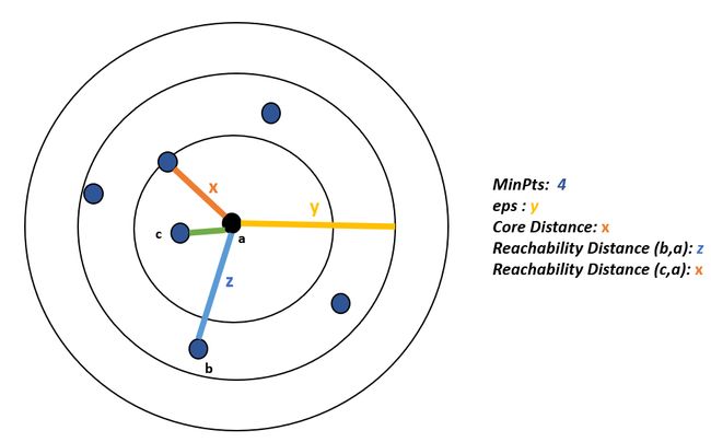
Core point: A point that resides at the center of the cluster can be accepted as a core point by providing minimally MinPts data points are located within its neighbors.
核心点:通过提供最少的MinPts数据点位于其邻居内,可以将位于群集中心的点视为核心点。
Core Distance: The minimum length of radius required to group provided observations as a core point.
核心距离:将提供的观测值分组为核心点所需的最小半径长度。
Reachability Distance: This distance metric represents the shortest length that is defined with respect to the cluster’s central point to another data point which cannot be smaller than the core distance. In the below depiction, the reachability distance between (c, a) is assigned as x, since their distance is smaller than the core distance which is not acceptable.
可达距离:此距离度量表示相对于群集中心点到另一个数据点的最短长度,该长度不能小于核心距离。 在下面的描述中, (c,a)之间的可到达距离被指定为x ,因为它们的距离小于不可接受的核心距离。
用于实现的Python库: (Python Library for Implementation:)
sklearn.cluster.OPTICS
sklearn.cluster.optics
算法: (Algorithm:)
OPTICS(DB, Epsilon, MinPts)
    for each observation Point in dataset DB
        Point.reachabilityDistance = UNDEFINED
    for each unprocessed point Point of DB
        Neighbors = getNeighbors(Point, Epsilon)
        assign Point as visited
        output Point to the ordered list
        if coreDistance(Point, Epsilon, MinPts) != UNDEFINED then
            Queue = empty priority queue
            updateCluster(Neighbors, Point, Queue, Epsilon, MinPts)
            for each next Q in Queue
                Neighbors' = getNeighbors(Q, Epsilon)
                assign Q as visited
                output Q to the ordered list
                if coreDistance(Q, Epsilon, MinPts) != UNDEFINED do
                    updateCluster(Neighbors', Q, Queue, Epsilon, MinPts)updateCluster(N, Point, Queue, Epsilon, MinPts) is
    coreDist = coreDistance(Point, Epsilon, MinPts)
    for each Observation in N
        if Observation is not visited then
            newReachabilityDistance = max(coreDist, dist(Point, Observation))
            if Observation.reachabilityDistance == UNDEFINED then
                Observation.reachabilityDistance = newReachabilityDistance
                Queue.insert(Observation, newReachabilityDistance)
                if newReachabilityDistance < Observation.reachabilityDistance then
                    Observation.reachabilityDistance = newReachabilityDistance
                    Queue.moveObservation(Observation, newReachabilityDistance)
3.基于距离的方法 (3. DISTANCE-BASED APPROACHES)
3.1。 局部离群因子(LOF) (3.1. Local Outlier Factor (LOF))
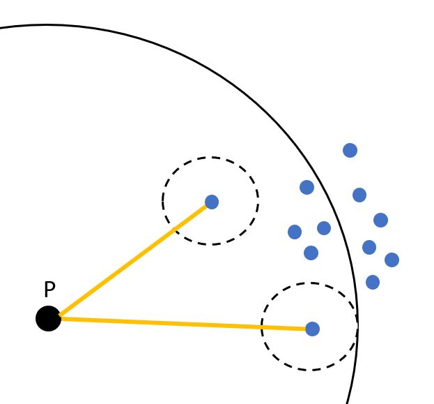
The Local Outlier Factor can be described as the calculation that scans through the neighbors of a certain point to discover its density and examine this to the density of other points to measure the distance between them.
可以将局部离群因子描述为一种计算,该计算将扫描某个点的邻居以发现其密度,并将其检查到其他点的密度以测量它们之间的距离。
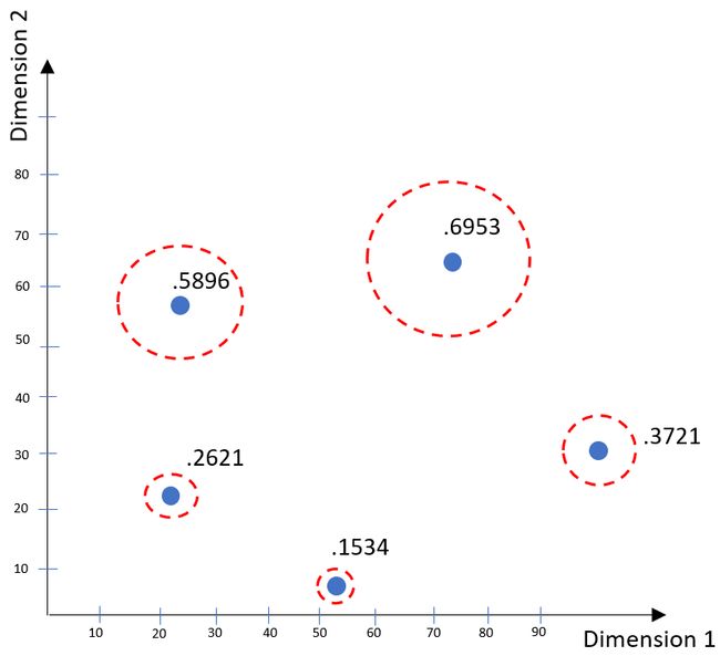
It calculates a score matching the degree of irregularity of the observations and measures the local density differentiation of a specified data point comparing to its neighbors. The logic is to identify the samples that have a considerably minor density than their surrounded-points.
它计算与观察结果的不规则程度相匹配的分数,并测量指定数据点与其相邻点的局部密度差异。 逻辑是识别密度比其包围点小得多的样本。
Figure 8. Point P has a higher LOF score since its density is lower than its surrounded densities. (Image by the author) 图8. 点P的LOF得分较高,因为其密度低于其周围的密度。 (作者提供的图片)Inlier points are local in the local outlier factor score builds upon how detached a single data node is regarding the encircling region. More accurately, the condition of being local is assigned by k-nearest neighbors, whose gap between points is used to calculate the local density.
内在点在本地离群因素评分中是本地的,这取决于单个数据节点与周围区域的分离程度。 更准确地说,存在局部的条件由k个最近的邻居分配,其点之间的间隙用于计算局部密度。
By contrasting the inner density of a point to the local densities of its neighbors, one can specify samples which allocates a distinctively lower density than their neighbors can be called as outliers.
通过将一个点的内部密度与其邻居的局部密度进行对比,可以指定分配明显低于其邻居的密度的样本(称为异常值)。
Figure 9. LOF score visualization. (Image by the author) 图9. LOF分数可视化。 (图片由作者提供)用于实现的Python库: (Python Library for Implementation:)
sklearn.neighbors.LocalOutlierFactor
sklearn.neighbors.LocalOutlierFactor
算法: (Algorithm:)
LOF = null
for each observation Point in DB
    KNNeighbors = kDistance(Distance, K)
    LocalReacbilityDistance = reachDistanceK(KNNeighbors, K)
    for each Point in KNNeighbors
        tempLOF[i] = sum((LocalReacbilityDistance[Obs ∈ N (Point)])   /  LocalReacbilityDistance[i]) / |N(Point)|
        LOF =  max(LOF, tempLOF)
return top(LOF)
3.2。 具有局部异常因素的新颖性检测 (3.2. Novelty Detection with Local Outlier Factor)
Novelty detection can be accepted as the description of a novel (new) or undiscovered patterns in the data. The novelties revealed are not considered as anomalous data points; instead, they are been practiced to the data model.
新颖性检测 可以接受作为对数据中新颖(新)或未发现模式的描述。 所揭示的新颖性不被视为异常数据点; 而是将它们实践到数据模型中。
The complicatedness of present highly integrated systems is similar to a restricted comprehension of the connections between the different system components that can be collected. An unavoidable effect of this situation is the presence of an enormous number of potential unusual forms, some of which may not be established as rational which causes regular multi-class classification schemes improper for these operations. A possible resolution to this issue is proposed by the algorithm of novelty detection, in which a definition of being an inlier is trained by creating a model with various examples depicting positive states. Formerly undiscovered patterns are then tested by contrasting them with the model of accepted-inliers, usually proceeded in some mode of novelty score. A novelty score may be generated for these formerly unseen data points with the help of a decision threshold score. The points which substantially diverge from this decision threshold may be treated as outliers.
当前高度集成的系统的复杂性类似于对可收集的不同系统组件之间的连接的有限理解。 这种情况的不可避免的后果是存在大量潜在的异常形式,其中某些形式可能无法确定为合理形式,从而导致常规的多类分类方案不适用于这些操作。 通过新颖性检测算法提出了解决此问题的可能方法,其中通过创建一个模型来训练一个内部人的定义,该模型带有各种描述正状态的示例。 然后,通过将先前未发现的模式与可接受的内部模式进行对比来测试这些模式,通常以某种新颖性评分模式进行处理。 借助于决策阈值分数,可以为这些以前看不见的数据点生成新奇分数。 实质上偏离该决策阈值的点可被视为离群值。
In other words, novelty detection can be described as the process of acknowledging that test data deviates in some way from the training data. Its practical influence and challenging essence have guided many suggestions for being proposed. These approaches are mostly applied to datasets in which a huge number of cases of the inlier or positive state is available and where there are scarce data to define outlier or negative state.
换句话说,新颖性检测 可以描述为确认测试数据以某种方式偏离训练数据的过程。 它的实际影响力和挑战性本质引导了许多建议被提出。 这些方法大多应用于数据集,其中所述巨大或内点正状态的病例数可用,并且其中存在稀少数据来定义异常值或负状态。
Figure 10. One-class (left) and multi-class (right) novelty detection. (Image by the author) 图10.一类(左)和多类(右)新颖性检测。 (图片由作者提供)用于实现的Python库: (Python Library for Implementation:)
sklearn.neighbors.LocalOutlierFactor
sklearn.neighbors.LocalOutlierFactor
3.3。 马氏距离 (3.3. Mahalanobis Distance)
For the given data source that holds standard normal distribution, the corresponding mean shall be zero while variance shall be observed as 1.
对于保持标准正态分布的给定数据源,相应的平均值应为零,而方差应观察为1。
The standard normal distribution has differentiative specifications from the normal distribution that can be expressed by means of the normal distribution having two distinct parameters as μ=0 and σ=1 with a representation of N(μ,σ) → N(0,1).
的标准正态分布具有从分化规格正态分布可以由来表示正态分布 具有两个不同的参数,分别为μ= 0和σ= 1 ,表示为N(μ,σ)→N(0,1) 。
Figure 11. Normal Distribution (left) vs Standard Normal Distribution (right). (Image by the author) 图11.正态分布(左)与标准正态分布(右)。 (图片由作者提供)Mahalanobis Distance is one of the outlier detection approaches which provides a simple means of detecting outliers in multidimensional data where the distance is between a point and a distribution and not between two distinct points.
马氏距离是离群值检测方法之一,它提供了一种检测多维数据中离群值的简单方法,其中距离在一个点和一个分布之间,而不是在两个不同的点之间。
Figure 12. A point and a distribution. (Image by author) 图12.点和分布。 (作者提供的图片)用于实现的Python库: (Python Library for Implementation:)
sklearn.neighbors.DistanceMetric
sklearn.neighbors.DistanceMetric
算法: (Algorithm:)
First Version:

Mahalanobis = [(Y – X)T * SampCov -1 * (Y – X)] ^ 0.5- X, Y    : Pair of observations
- SampCov : Sample covariance matrixAlternative Version:

Distance_n = [((xn – x̄)^t)*(C)^(-1) * (xn – x̄)] ^ 0.5

- xn = an observation vector
- x̄ = arithmetic mean vector
4.基于隔离的方法 (4. ISOLATION-BASED APPROACH)
4.1。 隔离林 (4.1. Isolation Forest)
Isolation Forest also called iForest recognizes abnormal activities as opposed to profiling typical data points. Isolation Forest, similar to any tree ensemble methodology, is based on decision trees. Among these trees, partitions are generated by first arbitrarily choosing a component and afterward choosing a randomly selected value in the scope of min and max of in a specified feature set. The algorithm is based on the idea that outliers represent data points that are few and different.
隔离林 也称为iForest,它可以识别异常活动,而不是分析典型数据点。 类似于任何树集成方法,隔离林都基于决策树。 在这些树中,首先通过任意选择一个组件,然后在指定特征集中的min和max of范围内随机选择一个值来生成分区。 该算法基于离群值表示很少且不同的数据点的思想。
There exist two variables in this algorithm. One is the number of trees to be built and the size of sub-sampling which enables the following subjects:
该算法中存在两个变量。 其中之一是要建造的树木数量和子采样的大小,可实现以下主题:
(i) to accomplish a low time-complexity with a reduced memory necessity (ii) to carry out the impacts of swamping, labeling nonoutlier as an outlier, and masking, an unidentified outlier
(i)实现低时间复杂度并减少存储需求(ii)进行沼泽化,将非异常值标记为异常值以及掩盖未识别的异常值的影响
With the help of these parameters, the isolation forest method does not take into consideration the distance and density metrics to catch anomalous behavior. This approach adds an advantage to iForest over distance-centered or density-centered methodologies since it excludes an extensive load of distance measurement.
在这些参数的帮助下,隔离林方法不考虑距离和密度度量来捕获异常行为。 与以距离为中心或以密度为中心的方法相比,此方法为iForest添加了一个优势,因为它排除了大量的距离测量负担。
Isolation forest works very efficiently in case of having a narrow-sized data set to profile outliers.
如果使用狭窄的数据集来描述离群值,隔离林将非常有效地工作。
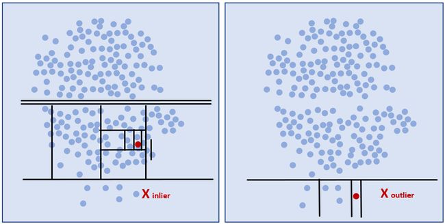
Below, the left-hand side graph shows the formed tree after the algorithm is executed. The blue line represents the normal data points while the red line can be accepted as the tree with anomalous data points. On the second graph, a schematic example of a tree and a plotted forest is shown with red-colored lines out abnormal data point existence while blue ones are normal ones.
下面,左侧图显示了执行算法后形成的树。 蓝线代表正常数据点,而红线可以被接受为具有异常数据点的树。 在第二张图上,以红色线条表示一棵树和一个绘制的森林的示意图,其中红色线条表示存在异常数据点,而蓝色线条表示正常数据点。
Figure 13. Isolation Forest visualization with outlier and inlier points. (Image by the author) 图13.带有离群点和离群点的Isolation Forest可视化。 (图片由作者提供)4.2。 公式: (4.2. Formulation:)
Step 1: Sampling for training a model Step 2: Random selection of a value that is between minimum and maximum of chosen data pointsStep 3: Repeating of step 2 of binary splitting to continue create a forestStep 4: Continuous feed of data resource to calculate anomaly score for every generated tree and their corresponding average path lengths
步骤1:为训练模型进行抽样步骤2:随机选择一个介于所选数据点的最小值和最大值之间的值。步骤3:重复执行二进制拆分的步骤2以继续创建林步骤4:将数据资源连续馈入计算每个生成的树的异常分数及其相应的平均路径长度
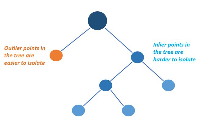
At the end of the average path sizes, an outlier is expected to have a shorter path length compared to an inlier.
在平均路径大小的结尾,离群值比离群值要短。
Figure 14. Average steps to generate an isolation forest by detecting inliers and outliers. (Image by the author) 图14.通过检测离群值和离群值来生成隔离林的平均步骤。 (图片由作者提供)用于实现的Python库: (Python Library for Implementation:)
sklearn.ensemble.IsolationForest
sklearn.ensemble.IsolationForest
算法: (Algorithm:)
t = null (the empty tree)if numberOfRow(Leaf) == 1 then return t
   Randomly select li a feature of Leaf
   Randomly select a split observation O ∈ (min(li), max(li))
   Add to t the node N li,Point
   Assign Leaf_l and Leaf_R as the matrix
   Repeat the looping with Leaf = Leaf_l
     Add the obtained tree as the left child of main tree t
   Repeat the looping with Leaf = Leaf_r
     Add the obtained tree as the right child of main tree t
5.基于分类的方法 (5. CLASSIFICATION-BASED APPROACHES)
5.1。 一类SVM (5.1. One-Class SVM)
The One-Class SVM can be accepted as sensitive to anomalous points which leads to poor performance outlier detection by using the training data with outliers. This predictor is correctly matched for novelty detection when the training set is not surrounded by outlier data points which aim to detect new observation as an outlier instead of detecting the noisy data in the existing data.
可以将一类SVM对异常点敏感,这可以通过将训练数据与离群值结合使用,从而导致较差的离群值检测。 当训练集没有被异常数据点包围时,该预测变量正确匹配以进行新颖性检测,该异常数据点旨在将新的观测值检测为异常值,而不是检测现有数据中的嘈杂数据。
A One-Class SVM might give beneficial results in multi-dimensional situations depending on the value of its hyperparameters. The aim of this algorithm to detach data points from the origin to maximize the distance between the subspace dimension to the origin.
一类SVM根据其超参数的值在多维情况下可能会产生有益的结果。 该算法的目的是将数据点与原点分离,以使子空间维度到原点之间的距离最大。
This situation proceeds in a result set of binary outputs which grab areas in the input space in which the probability density of the data locates.
这种情况在二进制输出的结果集中进行,该结果输出在输入空间中占据数据概率密度所在的区域。
In this way, the function returns +1 for inliers in a limited region which contains the space by occupying training observations and −1 for outliers.
通过这种方式,该函数通过占用训练观测值,对于包含空间的有限区域中的孤立点返回+1 ,而对于孤立点则返回-1 。
Figure 15. Outlier SVM Classifier with (1) for inliers, (-1) for outliers. (Image by the author) 图15.离群值SVM分类器,其中(1)代表离群值,(-1)代表离群值。 (图片由作者提供)用于实现的Python库: (Python Library for Implementation:)
sklearn.svm.OneClassSVM
sklearn.svm.OneClassSVM
算法: (Algorithm:)
X = {x1, x2....xm, z}, X ∈ R^d                # Observation VectorK(φ(xi), φ(xj ))                              # Feature Mapping
ρ = sum(k=1 to Ns) k=1 α(k) K(Φ(x̄)Φ(xk̄))    # Bias calculation
f(z̄) = sum(k=1 to Ns) k=1 α(k) K(Φ(xk̄)Φ(z̄))# Score Calculation

if f(z̄) > ρ then
   return 1
else
   return 0
end if
Questions and comments are highly appreciated!
问题和评论深表感谢!
6.参考 (6. References)
Anomaly Detection
异常检测
Identification of Outliers
异常值的识别
Isolation Forest
隔离林
Density-Based Spatial Clustering of Applications with Noise (DBSCAN)
基于密度的噪声应用空间聚类(DBSCAN)
OPTICS
光学
Local Outlier Factor
局部离群因子
Novelty Detection Local Outlier Factor
新奇检测局部离群因子
Mahalanobis Distance
马氏距离
One-Class SVM
一类SVM
Minimum Covariance Determinant
最小协方差行列式
翻译自: https://towardsdatascience.com/outlier-or-inlier-types-of-algorithms-to-detect-anomalous-behavior-ac15576823da
异常行为检测算法

