KAGGLE 比赛学习笔记---OTTO---baseline解读2

时间序列EDA-用户和实时会话
在Kaggle的Otto比赛中，“会话”一词实际上意味着“用户”。在本笔记本中，我们将显示用户及其实时会话时间序列EDA。我们观察到用户呈现出会话行为的常规模式。这些观察可以帮助我们为用户描述和设计特征。这些观察还可以让我们深入预测未来的点击、购物车和订单行为。我们将使用RAPID cuDF处理数据帧，使用matplotlib显示EDA。这里有关于这个笔记本的Kaggle讨论

# LOAD LIBRARIES
import pandas as pd, numpy as np
import matplotlib.pyplot as plt
import matplotlib.patches as mpatches
import cudf, cupy
print('Using RAPIDS version',cudf.__version__)


# LOAD TRAIN DATA. RANDOM SAMPLE 10%
train = cudf.read_parquet('../input/otto-full-optimized-memory-footprint/train.parquet')
sessions = train.session.unique()
sample = cupy.random.choice(sessions,len(sessions)//10,replace=False)
train = train.loc[train.session.isin(sample)]
print('We are using random 1/10 of users. Truncated train data has shape', train.shape )
train.head()





# MIN AND MAX TRAIN DATES
# IF USING ORIGINAL CSV, USE "TS * 1e6" BELOW
train.ts = cudf.to_datetime(train.ts * 1e9)
print('Train min date and max date are:', train.ts.min(),'and', train.ts.max() )
print('We will truncate train data to begin Aug 1st, 2022')
train = train.loc[train.ts >= cudf.to_datetime('2022-08-01')]






# COMPUTE DAY AND HOUR OF ACTIVITY
train['day'] = train.ts.dt.day
train['hour'] = train.ts.dt.hour
train = train.reset_index(drop=True)
# THE NEXT TWO LINES REPLICATE GROUPBY TRANSFORM
tmp = train.groupby('session').aid.agg('count').rename('n')
train = train.merge(tmp,on='session')
frequent_users = cupy.asnumpy( train.loc[train.n>40,'session'].unique() )
print(f"There are {len(frequent_users)} users whom each have over 40 item interactions in our truncated train data sample.")
print("We will display 128 of these most active users' behavior below.")








# COMPUTE USER REAL SESSIONS
train.ts = train.ts.astype('int64')/1e9
# THE NEXT THREE LINES REPLICATE GROUPBY DIFF
train = train.sort_values(['session','ts']).reset_index(drop=True)
train['d'] = train.ts.diff()
train.loc[ train.session.diff()!=0, 'd'] = 0
# IDENTITY REAL USER SESSIONS WHEN WE SEE 2 HOUR PAUSE IN ACTIVITY
train.d = (train.d > 60*60*2).astype('int8').fillna(0)
train['d'] = train.groupby('session').d.cumsum()









plt.hist(train.d.to_array(), bins=100)
plt.title("Histogram of Train Users' Real Session Count")
m = train.d.mean()
print(f'The mean session count per train user is {m:0.1f} with right skewed distribution below')
plt.show()





#Display User and Sessions Time Series
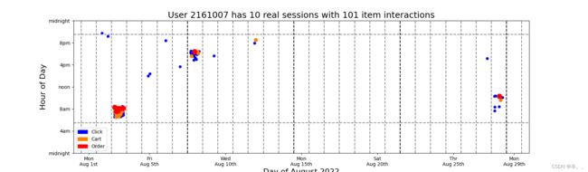
#Below we display a scatter plot with jitter. The x axis is day of the month August 2022. And the y axis is hour of the day. Many dots would fall on top of each other, so we add random x and y jitter. Also we color the clicks blue, carts orange, and orders red. We plot the clicks first, then carts, then orders. This guarentees that the orders and carts (when present) will always be visible and not be obscured by click dots




# DISPLAY USER ACTIVITY
colors = np.array( [(0,0,1),(1,0.5,0),(1,0,0)] )

for k in range(128):
    u = np.random.choice(frequent_users)
    tmp = train.loc[train.session==u].to_pandas()
    
    ss = tmp.d.max()+1
    ii = len(tmp)
    
    plt.figure(figsize=(20,5))
    for j in [0,1,2]:
        s = 25
        if j==1: s=50
        elif j==2: s=100
        tmp2 = tmp.loc[tmp['type']==j]
        xx = np.random.uniform(-0.3,0.3,len(tmp2))
        yy = np.random.uniform(-0.5,0.5,len(tmp2))
        plt.scatter(tmp2.day.values+xx, tmp2.hour.values+yy, s=s, c=colors[tmp2['type'].values])
    plt.ylim((0,24))
    plt.xlim((0,30))
    c1 = mpatches.Patch(color=colors[0], label='Click')
    c2 = mpatches.Patch(color=colors[1], label='Cart')
    c3 = mpatches.Patch(color=colors[2], label='Order')
    plt.plot([0,30],[6-0.5,6-0.5],'--',color='gray')
    plt.plot([0,30],[21+0.5,21+0.5],'--',color='gray')
    for k in range(0,30):
        plt.plot([k+0.5,k+0.5],[0,24],'--',color='gray')
    for k in range(1,5):
        plt.plot([7*k+0.5,7*k+0.5],[0,24],'--',color='black')
    plt.legend(handles=[c1,c2,c3])
    plt.xlabel('Day of August 2022',size=16)
    plt.xticks([1,5,10,15,20,25,29],['Mon\nAug 1st','Fri\nAug 5th','Wed\nAug 10th','Mon\nAug 15th','Sat\nAug 20th','Thr\nAug 25th','Mon\nAug 29th'])
    plt.ylabel('Hour of Day',size=16)
    plt.yticks([0,4,8,12,16,20,24],['midnight','4am','8am','noon','4pm','8pm','midnight'])
    plt.title(f'User {u} has {ss} real sessions with {ii} item interactions',size=18)
    plt.show()
    print('\n\n')









#    Observations
#We observe many patterns above. Most users exhibit regular behavior. They click, cart and order at the same hours each day. Also most users like to shop on the same days of the each week. Most users are active during the waking hours of day but some users like to shop during the night while others are sleeping. We also notice that users shop in clusters of activity. Our challenge in this competition is that we must both predict the remainder of the last cluster (provided in test data) and predict new clusters (after last timestamp in test). Furthermore all users in test data (not displayed in this notebook) have less than 1 week data, so we must predict user behavior given little user history information (i.e. the RecSys "cold start" problem). Understanding users and their behavior will help us predict test users' future behavior!

运行结果示例