锯齿波信号The sawtooth signal
lab里学到的代码和输出,说实话有些不懂但留着以后能翻查
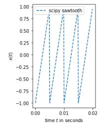
最简单的锯齿波
from scipy import signal
fs= 8000                   # sampling frequency
t = np.arange(0, 2, 1/fs)# ...       # time vector
f0 = 200                # frequency in Hz for scipy sawtooth
saw_tooth = signal.sawtooth(2 * np.pi * f0 * t)
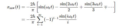
傅里叶级数和锯齿波

fs=8000 # sampling frequency

t=np.arange(0,2,1/fs) # time vector
f0=2                  # fundamental frequency in Hz
sin1=np.sin(2*np.pi*f0*t)
sin2=np.sin(2*np.pi*2*f0*t)/2
sin3=np.sin(2*np.pi*3*f0*t)/3
sin4=np.sin(2*np.pi*4*f0*t)/4
def generateSawTooth(f0=2, length = 2, fs=8000, order=10, height=1):
"""
Return a saw-tooth signal with given parameters.
Parameters
----------
f0 : float, optional
fundamental frequency $f_0$ of the signal to be generated,
default: 1 Hz
length : float, optional
length of the signal to be generated, default: 2 sec.
fs : float, optional
sampling frequency $f_s$, default: 8000 Hz
order : int, optional
number of sinosuids to approximate saw-tooth, default: 10
height : float, optional
height of saw-tooth, default: 1
Returns
-------
sawTooth
generated sawtooth signal
t
matching time vector
"""
t=np.arange(0,length,1/fs) # time vector
sum = np.zeros(len(t))
for ii in range(order):
jj=ii+1
sum += np.sin(2*np.pi*jj*f0*t)/jj
return 2*height*sum/np.pi, t
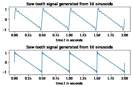
# generate a sawtooth signal composed of 10 sinusoids
saw,t = generateSawTooth(order=10)
plt.subplot(2,1,1)
plt.plot(t,saw)
plt.xlabel('time $t$ in seconds');
plt.title('Saw-tooth signal generated from 10 sinusoids')
# generate a sawtooth signal composed of 100 sinusoids
saw,t = generateSawTooth(order=100)
plt.subplot(2,1,2)
plt.plot(t,saw)
plt.xlabel('time $t$ in seconds');
plt.title('Saw-tooth signal generated from 10 sinusoids')
plt.tight_layout() # this allowes for some space for the title text.
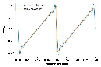
傅里叶级数和锯齿波(time-reverse)
def generateSawTooth2(f0=1, length = 2, fs=8000, order=10, height=1):
    """
    Return a saw-tooth signal with given parameters.

    Parameters
    ----------
    f0 : float, optional
        fundamental frequency $f_0$ of the signal to be generated,
        default: 1 Hz
    length : float, optional
        length of the signal to be generated, default: 2 sec.
    fs : float, optional
        sampling frequency $f_s$, default: 8000 Hz
    order : int, optional
        number of sinosuids to approximate saw-tooth, default: 10

    Returns
    -------
    sawTooth
        generated sawtooth signal
    t
        matching time vector
    """
    t=np.arange(0,length,1/fs)  # time vector
    sawTooth = np.zeros(len(t)) # pre-allocate variable with zeros
    for ii in range(1,order+1):
        sign = 2*(ii % 2) - 1# create alternating sign
        sawTooth += np.sin(2*np.pi*ii*f0*t)/ii
        #print(str(ii)+': adding ' + str(sign) + ' sin(2 $\pi$ '+str(ii*f0)+' Hz t)')
    return -2*height/np.pi*sawTooth, t

f0=1
saw2,t = generateSawTooth2(f0)
plt.plot(t,saw2,label='sawtooth Fourier')
plt.ylabel('$x_{\mathrm{saw}}(t)$')
plt.xlabel('time $t$ in seconds');

# compare to the sawtooth signal generated by scipy
saw_scipy = signal.sawtooth(2 * np.pi * f0 * t)

plt.plot(t, saw_scipy, '--', label='scipy sawtooth');
plt.legend();
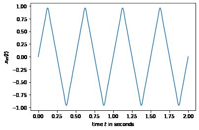
傅里叶级数和三角信号
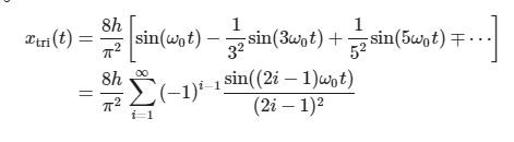
def generateTriangular(f0=2, length = 2, fs=8000, order=10, height=1):
    """
    Return a saw-tooth signal with given parameters.

    Parameters
    ----------
    f0 : float, optional
        fundamental frequency $f_0$ of the signal to be generated,
        default: 1 Hz
    length : float, optional
        length of the signal to be generated, default: 2 sec.
    fs : float, optional
        sampling frequency $f_s$, default: 8000 Hz
    order : int, optional
        number of sinosuids to approximate saw-tooth, default: 10
    height : float, optional
        height of saw-tooth, default: 1

    Returns
    -------
    sawTooth
        generated sawtooth signal
    t
        matching time vector
    """

    t=np.arange(0,length,1/fs) # time vector
    sum = np.zeros(len(t))
    for ii in range(1, order+1, 2):
        sign = -1* (ii % 4) + 2# create alternating sign
        print(str(ii)+': adding ' + str(sign) + ' sin(2 $\pi$ '+str(ii*f0)+' Hz t) / ' + str(ii**2))
        sum += sign*np.sin(2*np.pi*ii*f0*t)/(ii**2)
    return 8*height/(np.pi**2)*sum, t

# let's use the function and generate and plot a tringular wave form
f0=2
tri,t = generateTriangular(f0,order=10)
plt.plot(t,tri)
plt.ylabel('$x_{\mathrm{tri}}(t)$');
plt.xlabel('time $t$ in seconds');
傅里叶级数和方波
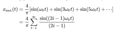
def generateSquare(f0=1, length = 2, fs=8000, order=10):
    t=np.arange(0,length,1/fs)  # time vector
    sum = np.zeros(len(t)) # pre-allocate variable with zeros
    for ii in range(1, order+1, 2):
        sum += np.sin(2*np.pi*ii*f0*t)/ii
        #print(str(ii)+': adding sin(2 $\pi$ '+str(ii*f0)+' Hz t)')
    return 4/np.pi*sum, t

# let's use the function and generate and plot a square wave form
f0=1 # desired frequency in Hz
rec,t = generateSquare(f0,order=20)
plt.plot(t,rec,label='square Fourier');
plt.ylabel('rectangular signal $x_{\mathrm{rect}}(t)$')
plt.xlabel('time $t$ in seconds');

# compare to the rectangular/square wave signal generated by scipy
rec_scipy = sig.square(2 * np.pi * f0 * t)
plt.plot(t,rec_scipy,'--',label='scipy square wave')
plt.legend();
