学习笔记 各种注意力机制 MSA, W-MSA, Local Attention,Stride Attention, ...
Computer Vision 里面的 Self-attention Head
queries, keys 和 values 的计算方式
queries, keys 和 values 是输入 I N × C I^{N\times C} IN×C 通过全连接层得到,具体如下:
queries Q N × d k = I N × C W Q N × d k Q^{N\times d_k}=I^{N\times C}W^{N\times d_k}_Q QN×dk=IN×CWQN×dk
keys K N × d k = I N × C W K N × d k K^{N\times d_k}=I^{N\times C}W^{N\times d_k}_K KN×dk=IN×CWKN×dk
values V N × d ′ = I N × C W V N × d ′ V^{N\times d^{\prime}}=I^{N\times C}W^{N\times d^{\prime}}_V VN×d′=IN×CWVN×d′
where the dimensions of query and key must be equal, which is d k d_k dk.
在 Vision Transformer 里, N = h w + 1 N=hw+1 N=hw+1,为输入图片 patches 的个数 + 一个用于分类的 token,为了方便,在以下的比较中,令 N = h w N=hw N=hw, 并且 d k d_k dk 和 d ′ d^{\prime} d′ 取作 C C C.
矩阵乘法的 Flop
M a × c = M a × b M b × c M^{a\times c}=M^{a\times b}M^{b\times c} Ma×c=Ma×bMb×c 的 Flop 为 a × b × c a\times b \times c a×b×c .
1. 单头 Self-attention
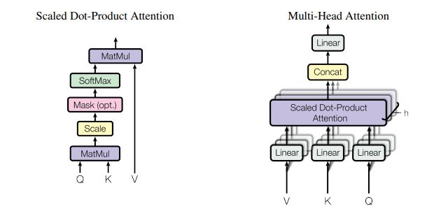
self-attention Attention ( Q , K , V ) = softmax ( Q K T d k ) V \displaystyle \operatorname{Attention}(Q, K, V)=\operatorname{softmax}\left(\frac{Q K^{T}}{\sqrt{d_{k}}}\right) V Attention(Q,K,V)=softmax(dkQKT)V
单头注意力模块的 Flop :
3 h w C 2 + ( h w ) 2 C + ( h w ) 2 C = 3 h w C 2 + 2 ( h w ) 2 3 h w C^{2}+(h w)^{2} C+(h w)^{2} C= 3 h w C^{2}+2(h w)^{2} 3hwC2+(hw)2C+(hw)2C=3hwC2+2(hw)2
2. Multi-Head Attention
原论文中每个 head 的获取方式是通过一个 linear project 得到的(全连接层),但是在实现中,正常直接通过对输入进行均分切片得到每一个 head 的输入,因此就省去了 W i { Q , K , V } W_{i}^{\{Q,K,V\}} Wi{Q,K,V} 三个全连接层的计算。直接简单均分切片奏效的原因,个人猜测是,网络很容易学到不同 head 所需要的模式应该位于输入 token 的哪几个维度上。以下是原论文的计算方式,这里不使用这种(linear project)计算方法。
Multi-head attention allows the model to jointly attend to information from different representation subspaces at different positions. With a single attention head, averaging inhibits this.
MultiHead ( Q , K , V ) = Concat ( head 1 , … , head h ) W O where head = Attention ( Q W i Q , K W i K , V W i V ) \begin{aligned} \operatorname{MultiHead}(Q, K, V) &=\operatorname{Concat}\left(\operatorname{head}_{1}, \ldots, \text { head }_{\mathrm{h}}\right) W^{O} \\ \text { where head } &=\operatorname{Attention}\left(Q W_{i}^{Q}, K W_{i}^{K}, V W_{i}^{V}\right) \end{aligned} MultiHead(Q,K,V) where head =Concat(head1,…, head h)WO=Attention(QWiQ,KWiK,VWiV)
Where the projections are parameter matrices W i Q ∈ R d model × d k , W i K ∈ R d model × d k , W i V ∈ R d model × d v W_{i}^{Q} \in \mathbb{R}^{d_{\text {model }} \times d_{k}}, W_{i}^{K} \in \mathbb{R}^{d_{\text {model }} \times d_{k}}, W_{i}^{V} \in \mathbb{R}^{d_{\text {model }} \times d_{v}} WiQ∈Rdmodel ×dk,WiK∈Rdmodel ×dk,WiV∈Rdmodel ×dv and W O ∈ R h d v × d model W^{O} \in \mathbb{R}^{h d_{v} \times d_{\text {model }}} WO∈Rhdv×dmodel .
直接使用简单均分切片的方法相较于多头注意力模块相比单头注意力模块的计算量仅多了最后一个融合矩阵 W O ∈ R h d v × d model W^{O} \in \mathbb{R}^{h d_{v} \times d_{\text {model }}} WO∈Rhdv×dmodel 的计算量 h w C 2 hwC^2 hwC2 , 所以多头注意力的 Flop 为(详细计算可参见这里):
3 h w C 2 + 2 ( h w ) 2 + h w C 2 = 4 h w C 2 + 2 ( h w ) 2 3 h w C^{2}+2(h w)^{2} +h w C^{2}=4 h w C^{2}+2(h w)^{2} 3hwC2+2(hw)2+hwC2=4hwC2+2(hw)2
3. Windowing Multi-Head Attention
假设每个 window 的大小为 M × M M\times M M×M,Windowing Multi-Head Attention 相当于在 M × M M\times M M×M 的窗口上做 h M × w M \displaystyle \frac{h}{M}\times \frac{w}{M} Mh×Mw 次Multi-Head Attention,因此所以Windowing Multi-Head Attention 的 Flop 为:
4 h w C 2 + 2 M 2 h w C 4 h w C^{2}+2 M^{2} h w C 4hwC2+2M2hwC
各式各樣神奇的自注意力機制 (Self-attention) 變型
Notice
- Self-attention is only a module in a larger network.
- Self-attention dominates computation when
Nis large. - Usually developed for image processing
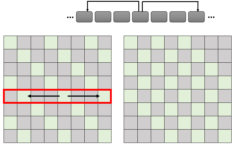
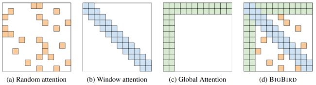
1. Local Attention / Truncated Attention
只考虑相邻 sequence 的 attention .
Self-attention 与 CNN 的区别之一为, self-attention 关注的范围更大,CNN 关注的范围只在局部。因此 Local Attention 在一定程度上抛弃了 self-attention 的优点,与 CNN 更为相似,因此 Local Attention 可以加快运算,但是在性能上不一定能带来提高。

2. Stride Attention
间隔一定的距离做 attention .
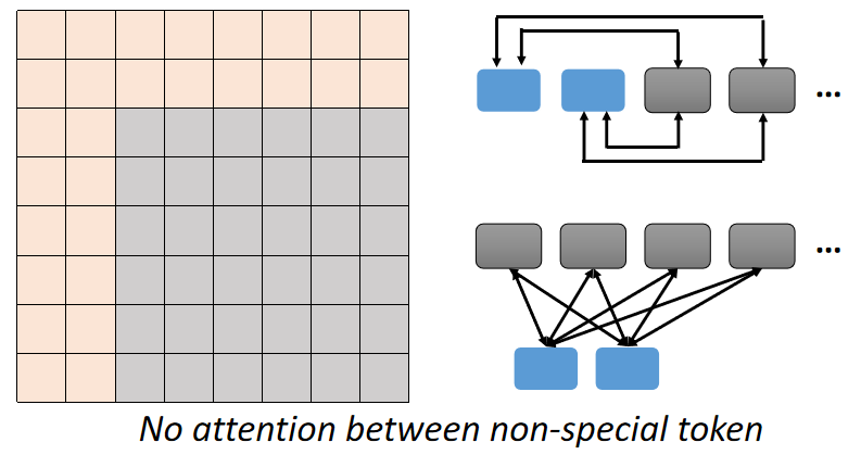
3. Global Attention
Add special token into original sequence
- Attend to every token → collect global information
- Attended by every token → it knows global information
How to choose the right Attention?
Different heads use different patterns.
- Longformer

- Big Bird
- Clustering Reformer & Routing Transformer


- Learnable Patterns Sinkhorn Sorting Network

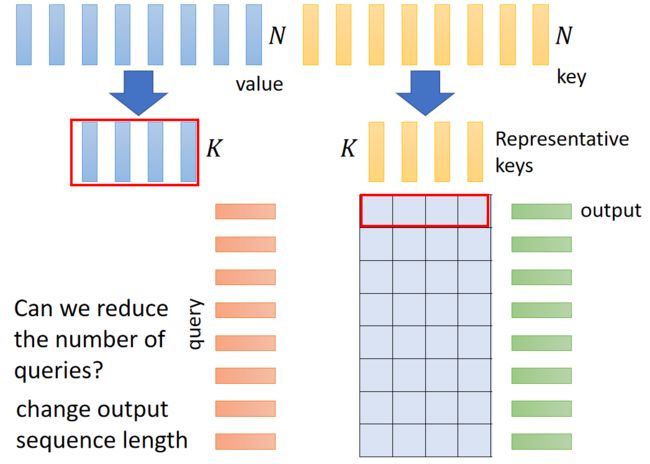
Do we need full attention matrix?
Linformer