吴恩达机器学习笔记(1)
1.监督学习的过程
将监督学习的数据集分为自变量(x)和因变量(y)。有监督学习算法的任务是,生成一个函数,将预测时需要用到的x输入进去,能输出相应的结果。
2.代价函数
以回归算法为例,设假设函数为 h θ ( x ) = θ 0 + θ 1 ∗ x h_\theta(x)=\theta_0+\theta_1*x hθ(x)=θ0+θ1∗x,代价函数(cost function)为 J ( θ 0 , θ 1 ) = 1 2 m ∑ i = 1 m ( h θ ( x ( i ) ) − y ( i ) ) J(\theta_0,\theta_1)=\frac{1}{2m}\sum_{i=1}^m(h_\theta(x^{(i)})-y^{(i)}) J(θ0,θ1)=2m1∑i=1m(hθ(x(i))−y(i)),则为了找到最适合的 θ 0 , θ 1 \theta_0,\theta_1 θ0,θ1,则应找到代价函数相应的最小值。
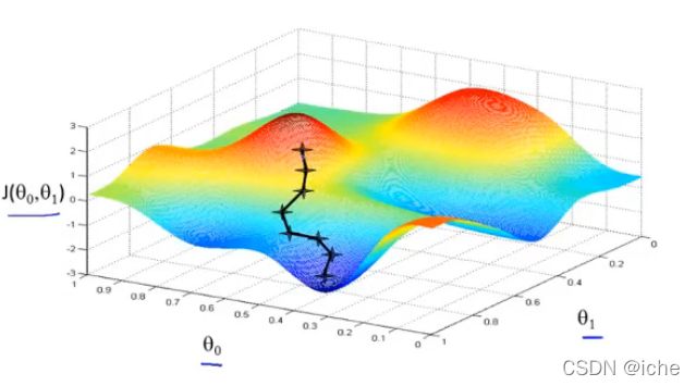
3.梯度下降
梯度下降Gradient descent是用来找到最适合的 θ 0 , θ 1 \theta_0,\theta_1 θ0,θ1的算法。通过计算代价函数的偏导数,找到 θ 0 , θ 1 \theta_0,\theta_1 θ0,θ1变化的方向,改变 θ 0 , θ 1 \theta_0,\theta_1 θ0,θ1,的值,从而使代价函数的值降到局部最低点。
for j=0 and j=1
θ j : = θ j − α ∂ ∂ θ j j ( θ 0 , θ 1 ) \theta_j:=\theta_j-\alpha\frac{\partial}{\partial \theta_j}j(\theta_0,\theta_1) θj:=θj−α∂θj∂j(θ0,θ1)
即
θ 0 : = θ 0 − α 1 m ∑ i = 1 m ( h θ ( x ( i ) ) − y ( i ) ) θ 1 : = θ 1 − α 1 m ∑ i = 1 m ( h θ ( x ( i ) ) − y ( i ) ) x ( i ) \theta_0:=\theta_0-\alpha\frac{1}{m}\sum_{i=1}^m(h_\theta(x^{(i)})-y^{(i)}) \\\theta_1:=\theta_1-\alpha\frac{1}{m}\sum_{i=1}^m(h_\theta(x^{(i)})-y^{(i)})x^{(i)} θ0:=θ0−αm1i=1∑m(hθ(x(i))−y(i))θ1:=θ1−αm1i=1∑m(hθ(x(i))−y(i))x(i)
α \alpha α是学习率learning rate,作用是控制我们以多大的幅度改变参数
4.多元线性回归
多元线性回归的参数相比于二元线性回归更多。假设函数 h θ ( x ) = θ 0 + θ 1 x 1 + θ 2 x 2 + … + θ n x n h_\theta(x)=\theta_0+\theta_1x_1+\theta_2x_2+…+\theta_nx_n hθ(x)=θ0+θ1x1+θ2x2+…+θnxn
对于上述情况,假设 x 0 = 1 x_0=1 x0=1,则有 h θ ( x ) = θ 0 x 0 + θ 1 x 1 + θ 2 x 2 + … + θ n x n h_\theta(x)=\theta_0x_0+\theta_1x_1+\theta_2x_2+…+\theta_nx_n hθ(x)=θ0x0+θ1x1+θ2x2+…+θnxn,define θ = [ θ 0 θ 1 ⋮ θ n ] \theta=\begin{bmatrix}\theta_0\\\theta_1\\\vdots\\\theta_n\end{bmatrix} θ=⎣⎢⎢⎢⎡θ0θ1⋮θn⎦⎥⎥⎥⎤, x = [ x 0 x 1 ⋮ x n ] x=\begin{bmatrix}x_0\\x_1\\\vdots\\x_n\end{bmatrix} x=⎣⎢⎢⎢⎡x0x1⋮xn⎦⎥⎥⎥⎤,则有 h θ ( x ) = θ ⊤ x h_\theta(x)=\theta^{\top}x hθ(x)=θ⊤x
Cost function: J ( θ ) = J ( θ 0 , θ 1 , … , θ n ) = 1 2 m ∑ i = 1 m ( h θ ( x ( i ) ) − y ( i ) ) J(\theta)=J(\theta_0,\theta_1,…,\theta_n)=\frac{1}{2m}\sum_{i=1}^m(h_\theta(x^{(i)})-y^{(i)}) J(θ)=J(θ0,θ1,…,θn)=2m1∑i=1m(hθ(x(i))−y(i))
Gradient descent:
f o r j = 0 , 1 , . . . , n θ j : = θ j − α ∂ ∂ θ j J ( θ ) = θ j − α 1 m ∑ i = 1 m ( h θ ( x ( i ) ) − y ( i ) ) x j ( i ) for\;j=0,1,...,n\\ \theta_j:=\theta_j-\alpha\frac{\partial}{\partial \theta_j}J(\theta) \\ =\theta_j-\alpha\frac{1}{m}\sum_{i=1}^m(h_\theta(x^{(i)})-y^{(i)})x^{(i)}_j forj=0,1,...,nθj:=θj−α∂θj∂J(θ)=θj−αm1i=1∑m(hθ(x(i))−y(i))xj(i)
多元线性回归梯度下降算法的优化
1.特征缩放
将特征向量中每个特征变量都缩放到相似区间内,从而使梯度下降更为精确和快速

特征变量除以最大值
均值归一化: x i = x i − μ i s i x_i=\frac{x_i-\mu_i}{s_i} xi=sixi−μi,其中 μ i \mu_i μi是 x i x_i xi的平均值, s i = m a x x i − m i n x i s_i=max_{x_i}-min_{x_i} si=maxxi−minxi是 x i x_i xi的范围
2.调整学习率 α \alpha α
如果 α \alpha α太小,那么代价函数收敛会很缓慢;如果 α \alpha α太大,那么代价函数可能会不收敛。
5.自定义特征和多项式回归
假如我们有一个房价数据集,里面包含房子的长和宽还有相应的房价。我们建立回归模型的时候,自变量不一定要局限于长和宽,我们可以自己定义一个特征 x = l e n g t h ∗ w i d t h x=length*width x=length∗width,用特征x来建立回归模型预测房价。
在比如说,现有数据集如下图
如图所示,该数据集并不适合做线性回归,这时候就可以考虑多项式回归。例如将特征变量设置为 s i z e size size和 s i z e \sqrt{size} size两个,即 h θ ( s i z e ) = θ 0 + θ 1 ∗ ( s i z e ) + θ 2 ∗ ( s i z e ) h_\theta(size)=\theta_0+\theta_1*(size)+\theta_2*(\sqrt{size}) hθ(size)=θ0+θ1∗(size)+θ2∗(size)
6.正规方程求解 θ \theta θ
set:
x ( i ) = [ x 0 ( i ) x 1 ( i ) x 2 ( i ) ⋮ x m ( i ) ] , X = [ ( x ( 1 ) ) ⊤ ( x ( 2 ) ) ⊤ ( x ( 3 ) ) ⊤ ⋮ ( x ( m ) ) ⊤ ] y = [ y ( 1 ) y ( 2 ) y ( 3 ) ⋮ y ( m ) ] x^{(i)}=\begin{bmatrix}x_0^{(i)}\\x_1^{(i)}\\x_2^{(i)}\\\vdots\\x_m^{(i)}\end{bmatrix}\;, X=\begin{bmatrix}(x^{(1)})^\top\\(x^{(2)})^\top\\(x^{(3)})^\top\\\vdots\\(x^{(m)})^\top\end{bmatrix} y=\begin{bmatrix}y^{(1)}\\y^{(2)}\\y^{(3)}\\\vdots\\y^{(m)}\end{bmatrix} x(i)=⎣⎢⎢⎢⎢⎢⎢⎡x0(i)x1(i)x2(i)⋮xm(i)⎦⎥⎥⎥⎥⎥⎥⎤,X=⎣⎢⎢⎢⎢⎢⎡(x(1))⊤(x(2))⊤(x(3))⊤⋮(x(m))⊤⎦⎥⎥⎥⎥⎥⎤y=⎣⎢⎢⎢⎢⎢⎡y(1)y(2)y(3)⋮y(m)⎦⎥⎥⎥⎥⎥⎤
则用以下公式即可求得最合适的 θ \theta θ值:
θ = ( X ⊤ X ) − 1 X ⊤ y \theta=(X^\top X)^{-1}X^\top y θ=(X⊤X)−1X⊤y
在处理线性回归问题时,如果要求的参数不多(小于1w),则用正规方程比较好。
在 θ \theta θ中所含的参数很多时用梯度下降更好。
其他更复杂模型的代价函数,有时候正规方程并不适用,此时也是梯度下降更好。
正规方程比较好。
在 θ \theta θ中所含的参数很多时用梯度下降更好。
其他更复杂模型的代价函数,有时候正规方程并不适用,此时也是梯度下降更好。