利用t-SNE对mnist数据集可视化

我把所有的过程全写入下面的代码注释中了。
主要流程有：

1. 将mnist数据集的64维转化为2维矩阵向量。（利用scikit-learn库中的TSNE库）
2. 将转化好的矩阵输出到二维空间中即可。

参考了官方的代码：scikit-learn/t-SNE

得到的结果如下图所示：

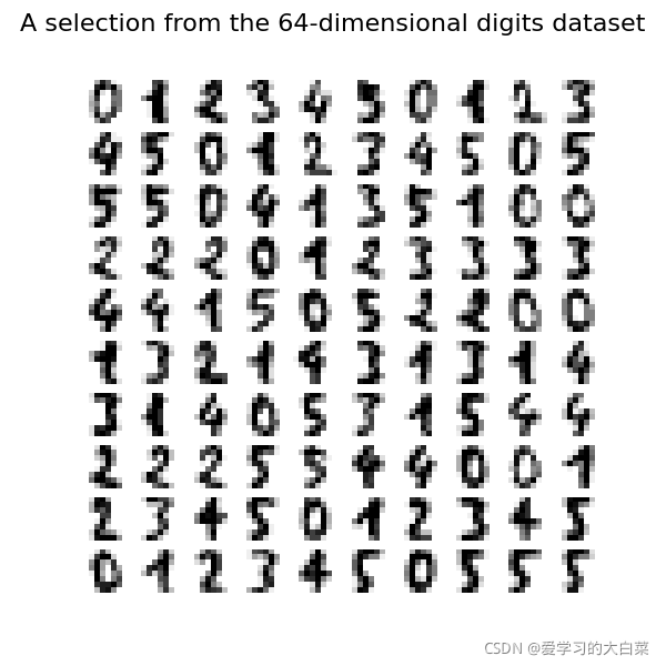
图1 选择Mnist数据集前100张图片

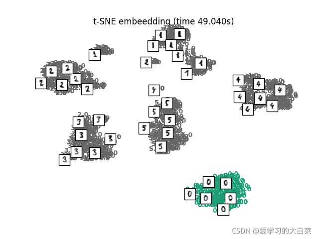
图2 用t-SNE可视化Mnist数据集前6种类

大约花了49s的时间，通过可视化发现每个样本降维后相同的类基本可以聚到一起。

代码如下：

# 1.引入数据库，取6种类。
from sklearn.datasets import load_digits

digits = load_digits(n_class=6)
X, y = digits.data, digits.target
n_samples, n_features = X.shape
n_neighbors = 30

# 2.展示100张mnist数据集图片
import matplotlib.pyplot as plt
fig, axs = plt.subplots(nrows=10, ncols=10, figsize=(6, 6))
for idx, ax in enumerate(axs.ravel()):
    ax.imshow(X[idx].reshape((8, 8)), cmap=plt.cm.binary)
    ax.axis("off")
_ = fig.suptitle("A selection from the 64-dimensional digits dataset", fontsize=16)
fig.show()

# 3.编写绘画函数，对输入的数据X进行画图。
import numpy as np
from matplotlib import offsetbox
from sklearn.preprocessing import MinMaxScaler


def plot_embedding(X, title, ax):
    X = MinMaxScaler().fit_transform(X)

    shown_images = np.array([[1.0, 1.0]])  # just something big
    for i in range(X.shape[0]):
        # plot every digit on the embedding
        ax.text(
            X[i, 0],
            X[i, 1],
            str(y[i]),
            color=plt.cm.Dark2(y[i]),
            fontdict={"weight": "bold", "size": 9},
        )

        # show an annotation box for a group of digits
        dist = np.sum((X[i] - shown_images) ** 2, 1)
        if np.min(dist) < 4e-3:
            # don't show points that are too close
            continue
        shown_images = np.concatenate([shown_images, [X[i]]], axis=0)
        imagebox = offsetbox.AnnotationBbox(
            offsetbox.OffsetImage(digits.images[i], cmap=plt.cm.gray_r), X[i]
        )
        ax.add_artist(imagebox)

    ax.set_title(title)
    ax.axis("off")

# 4.选择要用那种方式对原始数据编码(Embedding),这里选择TSNE。
#  n_components = 2表示输出为2维，learning_rate默认是200.0,
from sklearn.manifold import TSNE
embeddings = {
    "t-SNE embeedding": TSNE(
        n_components=2, init='pca', learning_rate=200.0, random_state=0
    ),
}

# 5.根据字典里（这里只有TSNE）的编码方式，生成压缩后的编码矩阵
# 即把每个样本生成了2维的表示。维度由原来的64位变成了2位。
# Input: (n_sample, n_dimension)
# Output: (n_sample, 2)

from time import time

projections, timing = {}, {}
for name, transformer in embeddings.items():
    if name.startswith("Linear Discriminant Analysis"):
        data = X.copy()
        data.flat[:: X.shape[1] + 1] += 0.01  # Make X invertible
    else:
        data = X

    print(f"Computing {name}...")
    start_time = time()
    print(data.shape, type(data.shape))
    data = data.astype(np.float)
    y = y.astype(np.float)
    projections[name] = transformer.fit_transform(data, y)
    timing[name] = time() - start_time



# 6.把编码矩阵输出到二维图像中来。
fig, ax = plt.subplots()
ax.axis("off")
title = f"{name} (time {timing[name]:.3f}s)"
plot_embedding(projections[name], title, ax)
plt.show()

附：t-SNE的一些参考链接：

1. https://lvdmaaten.github.io/tsne/
2. http://www.datakit.cn/blog/2017/02/05/t_sne_full.html
3. https://www.geeksforgeeks.org/how-to-add-a-legend-to-a-scatter-plot-in-matplotlib/