幕后产品_幕后逻辑回归

幕后产品

This is the second article in a series of articles where we will understand the “under the hood” workings of various ML algorithms, using their base math equations.

这是系列文章中的第二篇，我们将使用它们的基本数学方程式来理解各种ML算法的“幕后工作”。

1. Under the Hood — Linear Regression

   内幕下—线性回归

2. Under the Hood — Logistic Regression

   幕后-逻辑回归

With so many optimized implementations out there, we sometimes focus too much on the library and the abstraction it provides, and too little on the underlying calculations that go into the model. Understanding these calculations can often be the difference between a good and a great model.

由于存在许多优化的实现，因此有时我们过多地关注库及其提供的抽象，而很少关注模型中的基础计算。 理解这些计算通常可能是好的模型与好的模型之间的区别。

In this series, I focus on implementing the algorithms by hand, to understand the math behind it, which will hopefully help us train and deploy better models.

在本系列文章中，我专注于手工实现算法，以了解其背后的数学原理，这有望帮助我们训练和部署更好的模型。

Note — This series assumes you know the basics of Machine Learning and why we need it. If not, do give this article a read to get up to speed on why and how we utilize ML.

注—本系列假定您了解机器学习的基础知识以及我们为什么需要它。 如果不是，请阅读本文 ，以快速了解为什么以及如何利用ML。

逻辑回归 (Logistic Regression)

Logistic Regression builds on the concepts of Linear Regression, where the model produces a linear equation relating the input features(X) to the target variable (Y).

Logistic回归建立在线性回归的概念上，其中模型产生将输入要素(X)与目标变量(Y)关联的线性方程。

The two major differentiating features of the Logistic Regression algorithm are —

Logistic回归算法的两个主要区别特征是-

1. The target variable is a discrete value (0 or 1) unlike a continuous value, as in the case of Linear Regression, which adds an additional step after calculating output from the linear equation, to get discrete values.
   目标变量是与连续值不同的离散值(0或1)，例如在线性回归的情况下，它在计算线性方程的输出后增加了一个附加步骤，以获得离散值。
2. The equation built by the model focuses of separating the various discrete values of target — trying to identify a line such that all 1’s fall on one side of the line and all 0’s on the other.
   该模型建立的方程式着重于分离目标的各种离散值-试图识别一条线，使全1落在该线的一侧，而全0落在该线的另一侧。

Consider the following data, with two input features — X1, X2, and one binary (0/1) target feature — Y

考虑以下数据，其中包含两个输入功能-X1，X2和一个二进制(0/1)目标功能-Y

Logistic Regression will try to find the optimum values for the parameters w1, w2, and b, such that —

Logistic回归将尝试找到参数w1 ， w2和b的最佳值，从而使—

Here, the function H, also known as the activation function, converts the continuous output values of y to a discrete value. This will ensure that the equation is able to output a 1 or 0 similar to the input data.

在此，函数H (也称为激活函数)将y的连续输出值转换为离散值。 这将确保该方程能够输出类似于输入数据的1或0。

The algorithm finds these optimum values using the following steps —

该算法使用以下步骤找到这些最佳值-

0. Sample data containing binary(0,1) targets 0.包含二进制(0,1)目标的样本数据

1. Assign random values to w1, w2, and b.

   将随机值分配给w1 ， w2和b。

Assign random values to w1, w2 and b 为w1，w2和b分配随机值

2. Pick one instance of the data and calculate the continuous output (z).

2.选择一个数据实例并计算连续输出(z)。

Pick one instance and calculate z 选择一个实例并计算z

3. Calculate the discrete output (ŷ) using the activation function H().

3.使用激活函数H()计算离散输出(ŷ )。

H() to calculate ŷ H()计算ŷ

4. Calculate loss — Did our assumptions lead us close to a 1, when the actual target was 1?

4.计算损失-我们的假设是否使我们接近1，而实际目标是1？

Calculate loss 计算损失

5. Calculate the gradient for w1, w2 and b — How should we change the parameters to move closer to the actual output?

5.计算w1 ， w2和b的梯度-我们应如何更改参数以使其更接近实际输出？

6. Update w1, w2 and b.

6.更新w1 ， w2和b 。

Calculate gradient and update parameters 计算梯度并更新参数

7. Repeat steps 2–6 until convergence.

7.重复步骤2–6，直到收敛为止。

Repeat with another instance 对另一个实例重复

Let’s look at each of these steps in detail.

让我们详细了解这些步骤。

1.为w1，w2和b分配随机值 (1. Assign random values to w1, w2, and b)

We start with assigning random values to the model parameters —

我们从为模型参数分配随机值开始-

2. 选择一个数据实例并计算连续输出(z) (2. Pick one instance of the data and calculate the continuous output (z))

Let’s start with the first row of our data —

让我们从数据的第一行开始-

Putting in our assumed parameter values, we get —

输入假定的参数值，我们得到—

3. 使用激活函数H() 计算离散输出( ŷ )— (3. Calculate the discrete output (ŷ) using the activation function H() —)

If you’ve been following the “Under the Hood” series, you would have noticed that Steps 1 and 2 are exactly the same as in Linear Regression. This point will come up often, as Linear Regression forms the foundation for most algorithms out there — from simple ML algorithms to Neural Networks.

如果您一直遵循“高级知识”系列，则可能会注意到步骤1和步骤2与线性回归完全相同。 由于线性回归是目前大多数算法(从简单的ML算法到神经网络)的基础，因此这一点经常会提到。

It’s all powered by Y = MX + c

全部由Y = MX + c驱动

With our foundation laid out, we now focus on what makes Logistic Regression different from Linear Regression, and this is where the “activation function” comes in.

在奠定了基础的基础上，我们现在关注使Logistic回归与线性回归不同的原因，这就是“激活函数”出现的地方。

The activation function forms the bridge between the linear world with continuous target values and the “logistic” world (like the one we are working in right now!) with discrete target values.

激活函数在具有连续目标值的线性世界和具有离散目标值的“后勤”世界(就像我们现在正在研究的那样)之间架起了桥梁。

A simple form of an activation function would be a thresholding function (also known as the “Step function”) —

激活函数的简单形式是阈值函数(也称为“阶跃函数”)—

But, as with all things ML, “it can’t be that simple”.

但是，就像ML一样， “不可能那么简单” 。

One major flaw with a simple thresholding function like this, is that we have to manually select the right threshold(based on the range of output) every time we build a classification model. Our values could have any arbitrary range depending on the input variables and weights.

像这样的简单阈值功能的一个主要缺陷是，每次构建分类模型时，我们都必须手动选择正确的阈值(基于输出范围)。 根据输入变量和权重，我们的值可以具有任意范围。

Another fact working against a simple function like this, is that it is not differentiable at z=threshold. We need to follow the pipeline of loss -> gradient -> weight-update, hence we will need to make things a bit more complex here such that our life is simpler when we calculate the derivative(gradient) of our loss.

针对像这样的简单函数起作用的另一个事实是，在z = threshold处它是不可微的。 我们需要遵循损失-> 梯度 ->权重更新的流水线，因此我们需要在这里使事情变得更复杂，以便在计算损失的导数(梯度)时我们的生活更简单。

This is where a slightly modified version of the threshold — the Sigmoid function, comes in —

这是阈值的一个稍微修改的版本(Sigmoid函数)出现在此处-

Just like thresholding, the sigmoid function converts real number values, to a value between 0 and 1 with a midpoint at z=0 (thus solving our first problem). As evident from the graph, the function is smooth at all points, which will be of benefit when calculating gradients(thus solving our second problem).

就像阈值一样，S型函数将实数值转换为0到1之间的值，且中点为z = 0(从而解决了第一个问题)。 从图中可以明显看出，该函数在所有点上都是平滑的，这在计算梯度时将很有用(从而解决了我们的第二个问题)。

Another advantage of the sigmoid function is that it tells us how close our estimate is, to 0 or 1. This helps us get a good understanding of the model loss(error) — a prediction of 0.9 for a row that has an actual 1 is better than a prediction of 0.7. Such intricacies are lost when using a step function.

S形函数的另一个优点是，它告诉我们估算值接近0或1。这有助于我们更好地理解模型损失(错误)，对于实际值为1的行的预测为0.9，优于0.7的预测。 当使用步进功能时，这样的复杂性会丢失。

Let’s use the sigmoid function to calculate our estimated output —

让我们使用Sigmoid函数来计算我们的估计输出-

4. 计算损失 (4. Calculate loss)

Building on Linear Regression, we could choose squared error to represent our loss, but that would always make the error small, as our values lie in the 0–1 range. We need a function that outputs a large loss when our assumptions provide a value close to 0, while the actual is 1, and vice-versa.

在线性回归的基础上，我们可以选择平方误差来表示我们的损失，但这将使误差始终很小，因为我们的值在0–1范围内。 当我们的假设提供接近0的值，而实际为1时，我们需要一个输出大损失的函数，反之亦然。

One such function is the log-loss, which uses log transformation of our predicted output(z) to calculate loss.

对数损失就是这样一种功能，它使用我们的预测输出(z)的对数变换来计算损失。

We define the loss function as —

我们将损失函数定义为-

The output of the log function approaches negative infinity as the input reaches close to 0, and it is 0 when the input is 1. The negative sign inverts the log values to ensure our loss lies between 0 to infinity.

当输入接近0时，对数函数的输出接近负无穷大，而当输入为1时，对数输出为0。负号反转对数以确保损失在0到无穷大之间。

We can write the function as a single equation —

我们可以将函数写为一​​个方程式-

We can now calculate the error our assumptions lead us to —

现在，我们可以计算假设导致的误差-

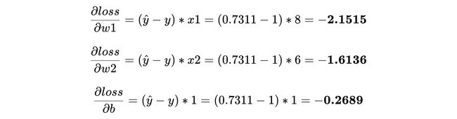
5. 计算w1，w2和b的梯度 (5. Calculate the gradient for w1, w2 and b)

We now calculate the impact each of our parameter has on the predicted output(and loss) by calculating the gradient of each of our parameters vs the loss.

现在，我们通过计算每个参数与损耗的梯度来计算每个参数对预测输出(和损耗)的影响。

This is where having differential functions in our pipeline make our life easy, giving us derivatives** for each of our parameters as —

在这里，我们的管道中具有微分功能，使我们的生活变得轻松，为我们的每个参数提供了导数**，例如-

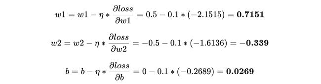
6. 更新w1，w2和b (6. Update w1, w2 and b)

The gradients tell us how much we should change each of our parameter assumptions to reduce the loss and move our predicted output closer to the actual output.

梯度告诉我们应改变多少参数假设以减少损耗并使预测输出更接近实际输出。

As we are “training” the model on one instance at a time, we want to limit the impact the loss on this individual instance has on our parameters. Thus, we scale the gradients to a tenth of their value, before updating the parameters, using “learning rate (η)” —

当我们一次在一个实例上对模型进行“训练”时，我们希望限制损失对单个实例的影响对我们的参数的影响。 因此，在使用“学习率( η) ”更新参数之前，我们将梯度缩放到其值的十分之一—

This completes one iteration of training.

这样就完成了一次迭代训练。

To get the optimum parameter values, we repeat the above steps either for a fixed number of times, or until our loss stops reducing i.e., convergence.

为了获得最佳的参数值，我们将上述步骤重复固定的次数，或者直到我们的损耗停止减小( 即收敛)为止。

Let’s work through another iteration, using the updated parameters —

让我们使用更新的参数来完成另一个迭代-

Looks like our loss has increased on this instance. This shows how the binary instances are pulling the weights in opposite direction to generate a decision boundary between the two classes.

看来我们在这种情况下的损失有所增加。 这显示了二进制实例如何沿相反方向拉权重以在两个类之间生成决策边界。

Repeating the steps for another few iterations*, sampling data randomly from the first 4 rows, we get the optimum weights as —

重复这些步骤再进行几次迭代*，从前4行中随机采样数据，我们得到的最佳权重为-

Using these values on our last row of data (which we did not use while training), we get —

在我们的最后一行数据中使用这些值(我们在训练时没有使用过)，我们得到-

That is really close to our actual class ‘1’.

这确实接近我们的实际等级“ 1”。

Choosing a cutoff at 0.5(mid-point of our sigmoid curve), gives us a prediction of 1 for this instance.

选择0.5(我们的S曲线的中点)的截止值，可以得到这种情况下1的预测。

And that’s it. At its core, this is all that the Logistic Regression algorithm does.

就是这样。 从本质上讲，这就是Logistic回归算法的全部工作。

这真的是Logistic回归的“全部”吗？ (Is this really “all” that Logistic Regression does?)

“Under the Hood” being the focus of this series, we took a look at the foundation of Logistic Regression taking one sample at a time and updating our parameters to fit the data.

本系列的重点是“内幕”，我们研究了Logistic回归的基础，一次采集了一个样本，并更新了参数以适合数据。

While it’s true that this is what Logistic Regression does at its core, there is a lot more that goes into a good Logistic Regression model, like —

虽然这确实是Logistic回归的核心工作，但好的Logistic回归模型还有很多其他功能，例如-

1. Regularization — L1 and L2

1.正则化-L1和L2

2. Learning Rate scheduling

2.学习率安排

3. Why choose sigmoid activation?

3.为什么选择S型激活？

4. Scaling and Normalizing variables

4.缩放和标准化变量

5. Multi-class classification

5.多类分类

I will cover these concepts in a parallel series focused on the various intricacies of the different ML algorithms we cover in this series.

我将在一个并行系列中介绍这些概念，重点关注我们在本系列中介绍的不同ML算法的各种复杂性。

下一步是什么？ (What’s next?)

In the next article in this series, we will continue with the classification task, and look under the hood of another class of algorithms — Decision Trees, which work a lot like how you and I would use reasoning to arrive at a conclusion regarding the data.

在本系列的下一篇文章中，我们将继续分类任务，并在另一类算法( 决策树)的背景下进行研究， 决策树的工作原理与您和我将如何使用推理得出有关数据的结论非常相似。 。

*Over 5 iterations, this is how our loss, gradients, and the parameter values changed —

*经过5次迭代，这就是我们的损耗，梯度和参数值的变化方式-

** I have not covered how we get the derivatives of our loss function w.r.t our parameters in this article, as the derivation is extensive and warrants an article in its own right (It will be covered in another article :))

** 我没有在本文中介绍如何通过参数获取损失函数的导数，因为推导范围很广，并有权利单独发表(将在另一篇文章中介绍：))

翻译自: https://towardsdatascience.com/under-the-hood-logistic-regression-407c0276c0b4

幕后产品