案例:线性回归-波士顿房价预测
python编程快速上手(持续更新中…)
文章目录
- python编程快速上手(持续更新中…)
-
- 数据介绍
- 1 分析
- 2 回归性能评估
- 3 线性回归-正规方程代码
- 4 线性回归-梯度下降代码
- 5 线性回归-岭回归代码
- 6.模型的保存和加载
数据介绍

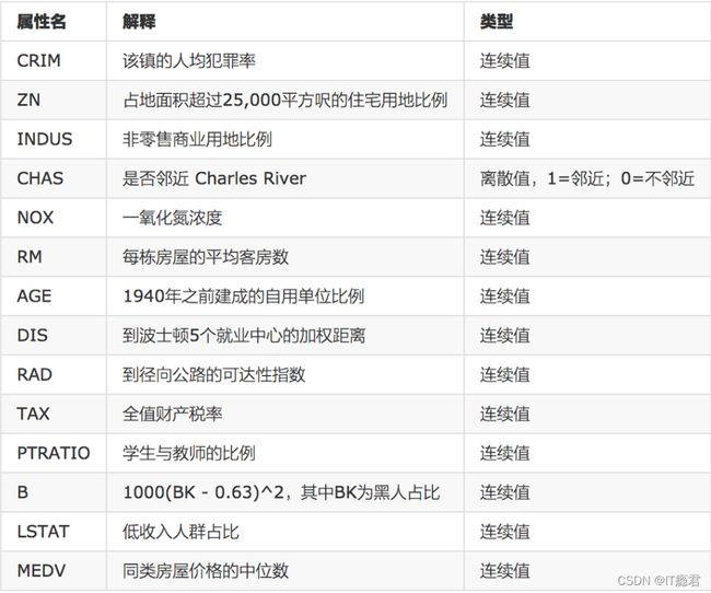
给定的这些特征,是专家们得出的影响房价的结果属性。我们此阶段不需要自己去探究特征是否有用,只需要使用这些特征。到后面量化很多特征需要我们自己去寻找
1 分析
回归当中的数据大小不一致,是否会导致结果影响较大。所以需要做标准化处理。
- 数据分割与标准化处理
- 回归预测
- 线性回归的算法效果评估
2 回归性能评估
均方误差(Mean Squared Error)MSE)评价机制:

注:yi为预测值,¯y为真实值
sklearn.metrics.mean_squared_error(y_true, y_pred)
- 均方误差回归损失
- y_true:真实值
- y_pred:预测值
- return:浮点数结果
3 线性回归-正规方程代码
from sklearn.datasets import load_boston
from sklearn.model_selection import train_test_split
from sklearn.preprocessing import StandardScaler
from sklearn.linear_model import LinearRegression
from sklearn.metrics import mean_squared_error

def linear_model1():
    """
    线性回归:正规方程
    :return:None
    """
    # 1.获取数据
    data = load_boston()

    # 2.数据集划分
    x_train, x_test, y_train, y_test = train_test_split(data.data, data.target, random_state=22)

    # 3.特征工程-标准化
    transfer = StandardScaler()
    x_train = transfer.fit_transform(x_train)
    x_test = transfer.fit_transform(x_test)

    # 4.机器学习-线性回归(特征方程)
    estimator = LinearRegression()
    estimator.fit(x_train, y_train)

    # 5.模型评估
    # 5.1 获取系数等值
    y_predict = estimator.predict(x_test)
    print("预测值为:\n", y_predict)
    print("模型中的系数为:\n", estimator.coef_)
    print("模型中的偏置为:\n", estimator.intercept_)

    # 5.2 评价
    # 均方误差
    error = mean_squared_error(y_test, y_predict)
    print("误差为:\n", error)


if __name__ == '__main__':
    linear_model1()
结果:
预测值为:
 [28.14790667 31.30481159 20.5173895  31.4803076  19.01576648 18.26058425
 20.57439825 18.45232382 18.46065155 32.93661269 20.3603692  27.24886071
 14.81691426 19.20872297 37.01503458 18.32036009  7.71389628 17.56196944
 30.18543811 23.60655873 18.14917545 33.84385342 28.48976083 16.9967041
 34.76065063 26.22246312 34.83857168 26.62310118 18.64402278 13.21154037
 30.37364532 14.70785748 37.18173708  8.88049446 15.06699441 16.14502168
  7.19990762 19.17049423 39.56848262 28.23663    24.62411509 16.75182833
 37.84465582  5.71770376 21.21547924 24.63882018 18.8561516  19.93416672
 15.19839712 26.29892968  7.4274177  27.14300763 29.18745146 16.27895854
  7.99799673 35.46394958 32.38905222 20.83161049 16.41464618 20.87141783
 22.92150844 23.60828508 19.32245804 38.33751529 23.87463642 18.98494066
 12.63480997  6.12915396 41.44675745 21.08894595 16.27561572 21.48546861
 40.74502107 20.4839158  36.82098808 27.0452329  19.79437176 19.64484428
 24.58763105 21.08454269 30.91968983 19.3326693  22.30088735 31.0904808
 26.36418084 20.25648139 28.81879823 20.82632806 26.01779216 19.37871837
 24.9599814  22.31091614 18.94468902 18.77414161 14.07143768 17.44450331
 24.19727889 15.86077811 20.09007025 26.51946463 20.1336741  17.02456077
 23.86647679 22.84428441 21.00754322 36.17169898 14.67959839 20.5656347
 32.46704858 33.24183156 19.81162376 26.55899048 20.90676734 16.42301853
 20.76605527 20.54658755 26.86304808 24.14176193 23.23824644 13.81640493
 15.37727091  2.79513898 28.89744167 19.80407672 21.50002831 27.5410586
 28.54270527]
模型中的系数为:
 [-0.64817766  1.14673408 -0.05949444  0.74216553 -1.95515269  2.70902585
 -0.07737374 -3.29889391  2.50267196 -1.85679269 -1.75044624  0.87341624
 -3.91336869]
模型中的偏置为:
 22.62137203166228
误差为:
 20.062193990359813
4 线性回归-梯度下降代码
def linear_model2():
    """
    线性回归:梯度下降法
    :return:None
    """
    # 1.获取数据
    data = load_boston()

    # 2.数据集划分
    x_train, x_test, y_train, y_test = train_test_split(data.data, data.target, random_state=22)

    # 3.特征工程-标准化
    transfer = StandardScaler()
    x_train = transfer.fit_transform(x_train)
    x_test = transfer.fit_transform(x_test)

    # 4.机器学习-梯度下降(特征方程)
    estimator = SGDRegressor(max_iter=1000)
    estimator.fit(x_train, y_train)

    # 5.模型评估
    # 5.1 获取系数等值
    y_predict = estimator.predict(x_test)
    print("预测值为:\n", y_predict)
    print("模型中的系数为:\n", estimator.coef_)
    print("模型中的偏置为:\n", estimator.intercept_)

    # 5.2 评价
    # 均方误差
    error = mean_squared_error(y_test, y_predict)
    print("误差为:\n", error)


if __name__ == '__main__':
	# 梯度下降
	linear_model2()
结果:
预测值为:
 [28.16765275 31.43568377 20.67624699 31.47873521 19.09529807 18.0916774
 20.71088456 18.43864496 18.54093415 32.86826544 20.55519266 27.09357369
 14.74707496 19.16830334 36.99158338 18.33559483  7.61381173 17.61316547
 30.3046187  23.71655995 17.96293231 33.85193239 28.31009475 16.83116214
 34.80591599 26.31718966 34.89368405 26.75272936 18.4560072  13.59729651
 30.37997441 14.07970664 37.51043297  8.80028654 15.12310142 15.90764702
  7.02272147 18.99193329 39.60117848 28.43595691 24.69486295 16.58456185
 37.77622064  5.45770871 21.0602221  24.62092354 18.78779232 19.90067394
 15.07921002 26.1559191   7.75253407 27.14464126 29.19504547 16.1037567
  7.7798851  35.47130656 32.28892234 21.37591334 16.41995997 20.88312904
 23.05731214 23.63385317 19.4375163  38.33232222 24.43687012 18.7796909
 12.44659051  5.88944976 41.45960491 21.1698849  16.07417249 21.53863881
 40.80581979 20.75202205 36.84797647 27.0908713  20.24446107 19.78613918
 24.69904782 21.75987895 31.15841813 19.37241052 22.27999078 31.26455517
 26.57529261 20.1147193  28.91256375 20.87740823 26.222995   18.77205383
 25.06836766 22.24603544 18.76067886 18.80686511 13.90201861 17.29385253
 24.20609951 15.66821147 19.88324949 26.53792947 19.93610232 16.84483492
 23.77279595 22.82952686 20.43793934 36.1597727  14.7404618  21.09618152
 32.55917975 33.05559837 19.82409528 26.28566981 20.86680778 16.59426603
 20.76137705 20.78602709 26.96640286 24.40313652 23.24801577 13.57641188
 15.2497289   2.53413597 29.01821637 19.62912672 21.61241239 27.6682532
 28.4334661 ]
模型中的系数为:
 [-0.61699261  1.08793005 -0.23640404  0.74634927 -1.93100072  2.73482427
 -0.11589056 -3.2634707   2.16405006 -1.49828302 -1.74879845  0.87978417
 -3.92112679]
模型中的偏置为:
 [22.62097918]
误差为:
 20.027424326908285
我们也可以尝试去修改学习率
estimator = SGDRegressor(max_iter=1000,learning_rate=“constant”,eta0=0.1)
此时我们可以通过调参数,找到学习率效果更好的值。
5 线性回归-岭回归代码
from sklearn.datasets import load_boston
from sklearn.model_selection import train_test_split
from sklearn.preprocessing import StandardScaler
from sklearn.linear_model import LinearRegression,SGDRegressor,Ridge,RidgeCV
from sklearn.metrics import mean_squared_error


def linear_model3():
    """
    线性回归:岭回归
    :return:
    """
    # 1.获取数据
    data = load_boston()

    # 2.数据集划分
    x_train, x_test, y_train, y_test = train_test_split(data.data, data.target, random_state=22)

    # 3.特征工程-标准化
    transfer = StandardScaler()
    x_train = transfer.fit_transform(x_train)
    x_test = transfer.fit_transform(x_test)

    # 4.机器学习-线性回归(岭回归)
    # estimator = Ridge(alpha=1)
    estimator = RidgeCV(alphas=(0.1, 1, 10))
    estimator.fit(x_train, y_train)

    # 5.模型评估
    # 5.1 获取系数等值
    y_predict = estimator.predict(x_test)
    print("预测值为:\n", y_predict)
    print("模型中的系数为:\n", estimator.coef_)
    print("模型中的偏置为:\n", estimator.intercept_)

    # 5.2 评价
    # 均方误差
    error = mean_squared_error(y_test, y_predict)
    print("误差为:\n", error)


if __name__ == '__main__':
    # 岭回归
    linear_model3()
预测值为:
 [28.01892316 31.10973232 20.71522003 31.27078503 19.35665239 18.27577089
 20.68537538 18.61236654 18.76244757 32.52583676 20.53950086 26.79920191
 14.90346898 19.32622055 36.73138795 18.1436293   8.34831679 17.80201281
 30.23022556 23.6588965  18.14940642 33.56719222 28.15659242 16.8342339
 34.43092768 25.95237531 34.29855907 26.67620464 18.53976338 14.28087185
 30.17681586 13.96270609 37.12398213  9.27914892 15.41928949 15.86636429
  7.41804801 18.98695207 39.26317607 28.49864203 24.65105363 16.86460045
 37.877637    5.73065641 20.91315988 24.38361983 19.22422747 20.0574593
 15.2017291  26.10094048  8.33736846 26.82949765 29.11129691 16.25679088
  8.29069659 35.08133644 31.5599828  21.72400461 16.61596806 21.0338388
 22.94263891 23.39788084 19.62635228 37.84115409 24.65810486 18.84971439
 12.9154527   6.11652874 41.31534803 21.13549069 15.93857105 21.79489742
 40.51105379 20.86424541 36.49859833 26.81086529 20.74647554 19.79398156
 24.67976477 22.38892245 30.97156138 19.38588583 22.36101941 30.98801612
 26.51755971 20.18795083 28.54818006 21.15792243 26.15395203 18.51365463
 24.67810928 22.20334022 18.98329801 19.19372987 14.29313106 17.38090659
 23.95558689 15.87908324 19.84135224 26.4365055  19.98310314 17.12864513
 23.61493568 22.67035994 20.13924313 35.61628002 15.04519051 21.33577802
 32.20782972 32.64268778 19.83978225 25.76604939 21.47552726 16.79428531
 20.79859329 20.90411594 26.88681963 24.47977682 23.10418168 13.64460207
 15.45039362  2.80255092 28.7074495  19.78868601 21.5465983  27.48968215
 28.05122649]
模型中的系数为:
 [-0.55638947  0.94868611 -0.29338303  0.76988373 -1.65228848  2.78456791
 -0.14333133 -2.94413876  1.84590375 -1.2436974  -1.68267802  0.86113858
 -3.76589168]
模型中的偏置为:
 22.62137203166228
误差为:
 20.170054477165934
6.模型的保存和加载
def load_dump_demo():
    """
    线性回归:岭回归
    :return:
    """
    # 1.获取数据
    data = load_boston()

    # 2.数据集划分
    x_train, x_test, y_train, y_test = train_test_split(data.data, data.target, random_state=22)

    # 3.特征工程-标准化
    transfer = StandardScaler()
    x_train = transfer.fit_transform(x_train)
    x_test = transfer.fit_transform(x_test)

    # 4.机器学习-线性回归(岭回归)
    # # 4.1 模型训练
    # estimator = Ridge(alpha=1)
    # estimator.fit(x_train, y_train)
    #
    # # 4.2 模型保存
    # joblib.dump(estimator, "./data/test.pkl")

    # 4.3 模型加载
    estimator = joblib.load("./data/test.pkl")

    # 5.模型评估
    # 5.1 获取系数等值
    y_predict = estimator.predict(x_test)
    print("预测值为:\n", y_predict)
    print("模型中的系数为:\n", estimator.coef_)
    print("模型中的偏置为:\n", estimator.intercept_)

    # 5.2 评价
    # 均方误差
    error = mean_squared_error(y_test, y_predict)
    print("误差为:\n", error)