用 Python 运行神经网络

一个神经网络类

我们在神经网络教程的前一章中学到了关于权重的最重要的事实。我们看到了它们的使用方式以及如何在 Python 中实现它们。我们看到，通过应用矩阵乘法，可以使用 Numpy 中的数组完成权重与输入值的乘法。

然而，我们没有做的是在真实的神经网络环境中测试它们。我们必须先创造这个环境。我们现在将在 Python 中创建一个类，实现一个神经网络。我们将分步进行，以便一切都易于理解。

我们班级需要的最基本的方法是：

• __init__ 初始化一个类，即我们将设置每一层的神经元数量并初始化权重矩阵。
• run：一种应用于我们想要分类的样本的方法。它将此样本应用于神经网络。我们可以说，我们“运行”网络以“预测”结果。此方法在其他实现中通常称为predict.
• train: 该方法获取一个样本和对应的目标值作为输入。如有必要，它可以通过此输入调整重量值。这意味着网络从输入中学习。从用户的角度来看，我们“训练”了网络。在sklearn例如，这种方法被称为fit

我们将把trainandrun方法的定义推迟到以后。权重矩阵应该在__init__方法内部初始化。我们是间接这样做的。我们定义一个方法create_weight_matrices并在__init__. 这样，init 方法就清晰了。

我们还将推迟向层添加偏置节点。

以下 Python 代码包含应用我们在前一章中得出的知识的神经网络类的实现：

导入 numpy的 是 NP
从 scipy.stats 导入 truncnorm

def  truncated_normal ( mean = 0 ,  sd = 1 ,  low = 0 ,  upp = 10 ): 
    return  truncnorm ( 
        ( low  -  mean )  /  sd ,  ( upp  -  mean )  /  sd ,  loc = mean ,  scale = sd )

类 神经网络：
   
    def  __init__ ( self ,  
                 no_of_in_nodes ,  
                 no_of_out_nodes ,  
                 no_of_hidden_​​nodes , 
                 learning_rate ): 
        self 。no_of_in_nodes  =  no_of_in_nodes 
        self 。no_of_out_nodes  =  no_of_out_nodes  
        self 。no_of_hidden_​​nodes  =  no_of_hidden_​​nodes 
        self 。learning_rate  =  learning_rate   
        self . create_weight_matrices ()
        
    def  create_weight_matrices ( self ): 
        rad  =  1  /  np 。SQRT （自我。no_of_in_nodes ）
        X  =  truncated_normal （平均值= 0 ， SD = 1 ， 低= -弧度， UPP =弧度）
        自我。weights_in_hidden  =  X 。RVS （（自我。no_of_hidden_​​nodes ， 
                                       自我。no_of_in_nodes )) 
        rad  =  1  /  np 。SQRT （自我。no_of_hidden_​​nodes ）
        X  =  truncated_normal （平均值= 0 ， SD = 1 ， 低= -弧度， UPP =弧度）
        自我。weights_hidden_​​out  =  X 。RVS （（自我。no_of_out_nodes ， 
                                        自我。no_of_hidden_​​nodes ））
           
    
    def  train ( self ):
        通过
    
    def  run ( self ):
        通过

我们不能用这段代码做很多事情，但我们至少可以初始化它。我们也可以看看权重矩阵：

simple_network  =  NeuralNetwork （no_of_in_nodes  =  3 ， 
                               no_of_out_nodes  =  2 ， 
                               no_of_hidden_​​nodes  =  4 ，
                               learning_rate  =  0.1 ）
打印（simple_network 。weights_in_hidden ）
打印（simple_network 。weights_hidden_​​out ）

输出：

[[-0.38364195 0.22655694 0.08684721]
 [ 0.2767437 0.28723294 -0.27309445]
 [ 0.25638328 -0.34340133 -0.37399997]
 [-0.1468639 0.54354951 0.08970088]]
[[ 0.34758695 0.41193854 -0.02512014 0.4407185 ]
 [ 0.21963126 0.37803538 0.40223143 0.13695252]]

激活函数、Sigmoid 和 ReLU

在我们对run方法进行编程之前，我们必须处理激活函数。我们在神经网络的介绍章节中有下图：

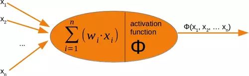
感知器的输入值由求和函数处理，然后是激活函数，将求和函数的输出转换为所需的更合适的输出。求和函数意味着我们将有一个权重向量和输入值的矩阵乘法。

神经网络中使用了许多不同的激活函数。可以在 Wikipedia 上找到对可能的激活函数的最全面的概述之一。

sigmoid 函数是常用的激活函数之一。我们使用的 sigmoid 函数也称为 Logistic 函数。

它被定义为

σ(X)=11+电子-X

让我们看一下 sigmoid 函数的图形。我们使用 matplotlib 绘制 sigmoid 函数：

import  numpy  as  np 
import  matplotlib.pyplot  as  plt 
def  sigma ( x ): 
    return  1  /  ( 1  +  np . exp ( - x ))

X  =  np 。linspace ( - 5 ,  5 ,  100 )


PLT 。绘图( X ,  sigma ( X ), 'b' ) 
plt 。xlabel ( 'X 轴' ) 
plt 。ylabel ( 'Y 轴' ) 
plt 。标题（'Sigmoid 函数' ）

PLT 。网格()

PLT 。文本( 2.3 ,  0.84 ,  r '$\sigma(x)=\frac {1} {1+e^{-x}}$' ,  fontsize = 16 )


PLT 。显示()

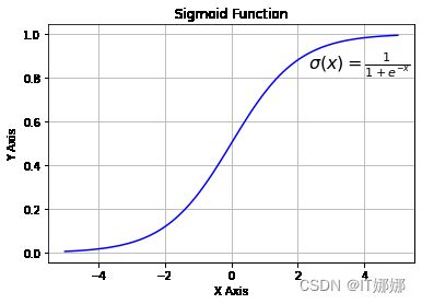
查看图表，我们可以看到 sigmoid 函数将给定的数字映射x到 0 到 1 之间的数字范围内。不包括 0 和 1！随着 的值x变大，sigmoid 函数的值越来越接近 1，随着xsigmoid 函数的值越来越小，sigmoid 函数的值越来越接近 0。

除了我们自己定义 sigmoid 函数之外，我们还可以使用来自 的 expit 函数scipy.special，它是 sigmoid 函数的一个实现。它可以应用于各种数据类，如 int、float、list、numpy、ndarray 等。结果是一个与输入数据 x 形状相同的 ndarray。

从 scipy.special 进口 expit
打印（expit （3.4 ））
打印（expit （[ 3 ， 4 ， 1 ））
打印（expit （NP 。阵列（[ 0.8 ， 2.3 ， 8 ]）））

输出：

0.9677045353015494
[0.95257413 0.98201379 0.73105858]
[0.68997448 0.90887704 0.99966465]

在神经网络中经常使用逻辑函数来在模型中引入非线性并将信号映射到指定的范围，即 0 和 1。它也很受欢迎，因为在反向传播中需要的导数很简单。

σ(X)=11+电子-X

及其衍生物：

σ′(X)=σ(X)(1-σ(X))

import  numpy  as  np 
import  matplotlib.pyplot  as  plt 
def  sigma ( x ): 
    return  1  /  ( 1  +  np . exp ( - x ))

X  =  np 。linspace ( - 5 ,  5 ,  100 )

PLT 。绘图（X ， 西格玛（X ））
plt 。绘图( X ,  sigma ( X )  *  ( 1  -  sigma ( X )))

PLT 。xlabel ( 'X 轴' ) 
plt 。ylabel ( 'Y 轴' ) 
plt 。标题（'Sigmoid 函数' ）

PLT 。网格()

PLT 。文本( 2.3 ,  0.84 ,  r '$\sigma(x)=\frac {1} {1+e^{-x}}$' ,  fontsize = 16 ) 
plt 。文本( 0.3 ,  0.1 ,  r '$\sigma \' (x) = \sigma(x)(1 - \sigma(x))$' ,  fontsize = 16 )


PLT 。显示()

我们还可以使用来自 numpy 的装饰器 vectorize 定义我们自己的 sigmoid 函数：

@np 。矢量化
DEF 乙状结肠（X ）：
    返回 1  /  （1  +  NP 。ë  **  - X ）

#sigmoid = np.vectorize(sigmoid) 
sigmoid ([ 3 ,  4 ,  5 ])

输出：

数组（[0.95257413，0.98201379，0.99330715]）

另一个易于使用的激活函数是 ReLU 函数。ReLU 代表整流线性单元。它也称为斜坡函数。它被定义为其论点的积极部分，即是=最大限度(0,X). 这是“目前，最成功和最广泛使用的激活函数是整流线性单元 (ReLU)” 1 ReLu 函数在计算上比 Sigmoid 类函数更高效，因为 Relu 意味着只选择 0 和参数 之间的最大值x。而 Sigmoids 需要执行昂贵的指数运算。

# 替代激活函数
def  ReLU ( x ): 
    return  np . 最大值( 0.0 ,  x )

# relu 的推导
def  ReLU_derivation ( x ): 
    if  x  <=  0 : 
        return  0 
    else : 
        return  1

导入 numpy 作为 np
导入 matplotlib.pyplot 作为 plt

X  =  np 。linspace （- 5 ， 6 ， 100 ）
PLT 。绘图( X ,  ReLU ( X ), 'b' ) 
plt 。xlabel ( 'X 轴' ) 
plt 。ylabel ( 'Y 轴' ) 
plt 。标题（'ReLU 函数' ）
plt 。网格() 
plt 。文本( 0.8 ,  0.4 , r '$ReLU(x)=max(0, x)$' ,  fontsize = 14 ) 
plt 。显示()

添加运行方法

我们现在拥有一切来实现我们的神经网络类的run（或predict）方法。我们将scipy.special用作激活函数并将其重命名为activation_function：

from  scipy.special  import  expit  as  activation_function

我们在该run方法中要做的所有事情包括以下内容。

1. 输入向量和 weights_in_hidden 矩阵的矩阵乘法。
2. 将激活函数应用于步骤 1 的结果
3. 步骤 2 的结果向量和 weights_in_hidden 矩阵的矩阵乘法。
4. 得到最终结果：将激活函数应用于 3 的结果

 从scipy.special import expit as activation_function from scipy.stats import truncnorm导入numpy 作为 np
     
   

def  truncated_normal ( mean = 0 ,  sd = 1 ,  low = 0 ,  upp = 10 ): 
    return  truncnorm ( 
        ( low  -  mean )  /  sd ,  ( upp  -  mean )  /  sd ,  loc = mean ,  scale = sd )


类 神经网络：
           
    def  __init__ ( self ,  
                 no_of_in_nodes ,  
                 no_of_out_nodes ,  
                 no_of_hidden_​​nodes , 
                 learning_rate ): 
        self 。no_of_in_nodes  =  no_of_in_nodes 
        self 。no_of_out_nodes  =  no_of_out_nodes 
        self 。no_of_hidden_​​nodes  =  no_of_hidden_​​nodes 
        self 。learning_rate  =  learning_rate  
        self . create_weight_matrices ()
        
    def  create_weight_matrices ( self ): 
        """ 一种初​​始化神经网络权重矩阵的方法""" 
        rad  =  1  /  np . SQRT （自我。no_of_in_nodes ）
        X  =  truncated_normal （平均值= 0 ， SD = 1 ， 低= -弧度， UPP =弧度）
        自我。weights_in_hidden  =  X 。房车（（自我。no_of_hidden_​​nodes ， 
                                       self 。no_of_in_nodes )) 
        rad  =  1  /  np 。SQRT （自我。no_of_hidden_​​nodes ）
        X  =  truncated_normal （平均值= 0 ， SD = 1 ， 低= -弧度， UPP =弧度）
        自我。weights_hidden_​​out  =  X 。RVS （（自我。no_of_out_nodes ， 
                                        自我。no_of_hidden_​​nodes ))
    
    
    def  train ( self ,  input_vector ,  target_vector ):
        通过
            
    
    def  run ( self ,  input_vector ): 
        """
        使用输入向量 'input_vector' 运行网络
        。'input_vector' 可以是元组、列表或 ndarray 
        """ 
        # 将输入向量转换为列向量
        input_vector  =  np 。数组（input_vector ， ndmin = 2 ）。T 
        input_hidden  =  activation_function ( self . weights_in_hidden  @  input_vector ) 
        output_vector  =  activation_function( self . weights_hidden_​​out  @  input_hidden )
        返回 output_vector
            

我们可以实例化这个类的一个实例，这将是一个神经网络。在以下示例中，我们创建了一个具有两个输入节点、四个隐藏节点和两个输出节点的网络。

simple_network  =  NeuralNetwork （no_of_in_nodes = 2 ， 
                               no_of_out_nodes = 2 ， 
                               no_of_hidden_​​nodes = 4 ，
                               learning_rate = 0.6 ）

我们可以将 run 方法应用于所有形状为 (2,) 的数组，以及具有两个数字元素的列表和元组。调用的结果由权重的随机值定义：

simple_network 。运行([( 3 ,  4 )])

输出：

数组([[0.62128186],
       [0.58719777]])

脚注

1拉马钱德兰，普拉吉特；巴雷特，佐夫；Quoc, V. Le（2017 年 10 月 16 日）。