【Python机器学习】层次聚类AGNES、二分K-Means算法的讲解及实战演示（图文解释 附源码）

需要源码和数据集请点赞关注收藏后评论区留言私信~~~

层次聚类

在聚类算法中，有一类研究执行过程的算法，它们以其他聚类算法为基础，通过不同的运用方式试图达到提高效率，避免局部最优等目的，这类算法主要有网格聚类和层次聚类算法

网格聚类算法强调的是分批统一处理以提高效率，具体的做法是将特征空间划分为若干个网格，网格内的所有样本看成一个单元进行处理，网格聚类算法要与划分聚类或密度聚类算法结合使用，网格聚类算法处理的单元只与网格数量有关，与样本数量无关，因此在数据量大时，网格聚类算法可以极大地提高效率

层次（Hierarchical）聚类算法强调的是聚类执行的过程，分为自底向上的凝聚方法和自顶向下的分裂方法两种。

凝聚方法是先将每一个样本点当成一个簇，然后根据距离和密度等度量准则进行逐步合并。

分裂方法是先将所有样本点放在一个簇内，然后再逐步分解。

前者的典型算法有AGNES算法，后者的典型算法有二分k-means算法。

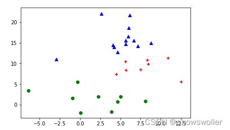
1：二分 k-means算法

二分k-means算法先将所有点看成一个簇，然后将该簇一分为二，之后选择其中一个簇继续分裂。选择哪一个簇进行分裂，取决于对其进行的分裂是否可以最大程度降低SSE值。如此分裂下去，直到达到指定的簇数目k为止

效果展示如下

 

部分代码如下 下面是分裂主循环代码

while len(SSE) < n_clusters:
    max_changed_SSE = 0
    tag = -1
    for i in range(len(SSE)): # 对每个簇进行试分簇，计算SSE的减少量
        estimator = KMeans(init='k-means++', n_clusters=2, n_init=n_init).fit(samples[i]) # 二分簇
        changed_SSE = SSE[i] - estimator.inertia_
        print(estimator.inertia_, ' - ', changed_SSE)
        if changed_SSE > max_changed_SSE: # 比较SSE值是不是减少了
            max_changed_SSE = changed_SSE
            tag = i
    # 正式分簇
    estimator = KMeans(init='k-means++', n_clusters=2, n_init=n_init).fit(samples[tag])
    indexs0 = np.where(estimator.labels_ == 0) # 标签为0的样本在数组中的下标
    cluster0 = samples[tag][indexs0] # 从簇中分出标签为0的新簇
    indexs1 = np.where(estimator.labels_ == 1)
    cluster1 = samples[tag][indexs1] # 从簇中分出标签为1的新簇
    
    del samples[tag]
    samples.append(cluster0)
    samples.append(cluster1)
    del SSE[tag]
    estimator = KMeans(init='k-means++', n_clusters=1, n_init=n_init).fit(cluster0)
    SSE.append(estimator.inertia_) # 新簇的SSE值
    estimator = KMeans(init='k-means++', n_clusters=1, n_init=n_init).fit(cluster1)
    SSE.append(estimator.inertia_)

 2：AGNES算法

AGNES（AGglomerative NESting）算法先将每个样本点看成一个簇，然后根据簇与簇之间的距离度量将最近的两个簇合并，一直重复合并到指定的簇数目k为止。

 

代码参数如下所示 

class sklearn.cluster.AgglomerativeClustering(n_clusters=2, affinity=’euclidean’, memory=None, connectivity=None, compute_full_tree=’auto’, linkage=’ward’, pooling_func=’deprecated’, distance_threshold=None)

n_clusters是指定的分簇数

linkage是簇距离度量方法，支持ward、complete、average和single四种方法。complete、average和single分别对应簇最大距离、簇平均距离和簇最小距离。

Ward方法与其它方法不一样，它不是按距离合并簇，而是合并使得偏差（样本点与簇中心的差值）平方和增加最小的两个簇。它先要对所有簇进行两两试合并，并计算偏差平方和的增加值，然后取增加最小的两个簇进行合并。

效果展示如下

部分代码如下

# Set up cluster parameters
plt.figure(figsize=(9 * 1.3 + 2, 14.5))
plt.subplots_adjust(left=.02, right=.98, bottom=.001, top=.96, wspace=.05,
                    hspace=.01)

plot_num = 1

default_base = {'n_neighbors': 10,
                'n_clusters': 3}

datasets = [
    (noisy_circles, {'n_clusters': 2}),
    (noisy_moons, {'n_clusters': 2}),
    (varied, {'n_neighbors': 2}),
    (aniso, {'n_neighbors': 2}),
    (blobs, {}),
    (no_structure, {})]

for i_dataset, (dataset, algo_params) in enumerate(datasets):
    # update parameters with dataset-specific values
    params = default_base.copy()
    params.update(algo_params)

    X, y = dataset

    # normalize dataset for easier parameter selection
    X = StandardScaler().fit_transform(X)

    # ============
    # Create cluster objects
    # ============
    ward = cluster.AgglomerativeClustering(
        n_clusters=params['n_clusters'], linkage='ward')
    complete = cluster.AgglomerativeClustering(
        n_clusters=params['n_clusters'], linkage='complete')
    average = cluster.AgglomerativeClustering(
        n_clusters=params['n_clusters'], linkage='average')
    single = cluster.AgglomerativeClustering(
        n_clusters=params['n_clusters'], linkage='single')

    clustering_algorithms = (
        ('Single Linkage', single),
        ('Average Linkage', average),
        ('Complete Linkage', complete),
        ('Ward Linkage', ward),
    )

    for name, algorithm in clustering_algorithms:
        t0 = time.time()

        # catch warnings related to kneighbors_graph
        with warnings.catch_warnings():
            warnings.filterwarnings(
                "ignore",
                message="the number of connected components of the " +
                "connectivity matrix is [0-9]{1,2}" +
                " > 1. Completing it to avoid stopping the tree early.",
                category=UserWarning)
            algorithm.fit(X)

        t1 = time.time()
        if hasattr(algorithm, 'labels_'):
            y_pred = algorithm.labels_.astype(int)
        else:
            y_pred = algorithm.predict(X)

        plt.subplot(len(datasets), len(clustering_algorithms), plot_num)
        if i_dataset == 0:
            plt.title(name, size=18)

        colors = np.array(list(islice(cycle(['#377eb8', '#ff7f00', '#4daf4a',
                                             '#f781bf', '#a65628', '#984ea3',
                                             '#999999', '#e41a1c', '#dede00']),
                                      int(max(y_pred) + 1))))
        plt.scatter(X[:, 0], X[:, 1], s=10, color=colors[y_pred])

        plt.xlim(-2.5, 2.5)
        plt.ylim(-2.5, 2.5)
        plt.xticks(())
        plt.yticks(())
        plt.text(.99, .01, ('%.2fs' % (t1 - t0)).lstrip('0'),
                 transform=plt.gca().transAxes, size=15,
                 horizontalalignment='right')
        plot_num += 1

plt.show()

 创作不易 觉得有帮助请点赞关注收藏~~~