从jieba分词到BERT-wwm——中文自然语言处理（NLP）基础分享系列（6）

第一个机器学习模型

上一回我们得到新闻标题文档的压缩到64维的LSI向量表示，我们用它来训练一个机器学习（Machine Learning）模型。
首先我们运行代码，重新在内存中加载它。

import pandas as pd 
import pickle 
from sklearn.feature_extraction.text import TfidfVectorizer 
 
pkl_file_rb = open(r'./save_file', 'rb') 
train =pickle.load(pkl_file_rb) 
 
corpus = pd.concat([train . title1_tokenized, train . title2_tokenized]) 
corpus = [c for c in corpus] 
 
tfidf_model = TfidfVectorizer().fit(corpus) 

matrix1= tfidf_model.transform(train['title1_tokenized']) 
matrix2= tfidf_model.transform(train['title2_tokenized']) 

from sklearn.decomposition import TruncatedSVD

svd_model = TruncatedSVD(n_components=64, algorithm='randomized', n_iter=100, random_state=122) #参数n_components即降维的目标维数r 
svd_model.fit(tfidf_model.transform(corpus))

matrix1_sub  = svd_model.transform(matrix1) 
matrix2_sub  = svd_model.transform(matrix2) 

我们把来自新闻标题A和B的LSI向量做一个差值，然后进行归一化处理。

from  sklearn import preprocessing 

input_data = matrix1_sub - matrix2_sub 
input_data = preprocessing.scale(input_data) 
input_data.shape 

(320552, 64)

将目标变量做数字化处理

我们已经将所有的新闻标题A和B以数字化表示，做成64维输入变量。
接下来需要将分类列 label 进行从文本到数字的转换。我们同样需要一个字典将分类的文字转换成索引。

# 定义每一个分类对应到的索引数字 
label_to_index = { 'unrelated' : 0 , 'agreed' : 1 , 'disagreed' : 2 } 

# 将分类标签对应到刚定义的数字
y_train_ = train . label . apply ( lambda x : label_to_index [ x ]) 
 
# y_train_ = np . asarray ( y_train_ ). astype ( 'float32' )  
print('y_train_.shape: ',y_train_.shape) 
y_train_ [11: 16 ] 

y_train_.shape:  (320552,)





id
10    1
13    1
12    1
15    0
17    2
Name: label, dtype: int64

切割训练数据集& 验证数据集

我们需要将整个训练数据集（Training Set）的多少比例切出来当作验证数据集（Validation Set）。此例中我们用10 %。
但为何要再把本来的训练数据集切成2 个部分呢？
一般来说，我们在训练时只会让模型看到训练数据集，并用模型没看过的验证数据集来测试该模型在真实世界的表现。（毕竟我们没有测试数据集的答案）

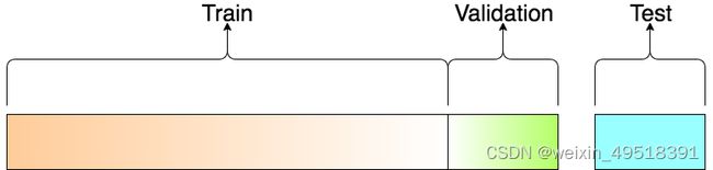
要切训练数据集/ 验证数据集，scikit-learn 中的 train_test_split 函数是一个不错的选择：

from sklearn import model_selection 
 
x_train, x_val, y_train, y_val = model_selection.train_test_split(input_data, y_train_, test_size = 0.1, random_state = 911) # 取10%做验证集 
 
print("Train Shape: {}".format(x_train.shape)) 
print("valid Shape: {}".format(x_val.shape)) 

Train Shape: (288496, 64)
valid Shape: (32056, 64)

训练机器学习模型

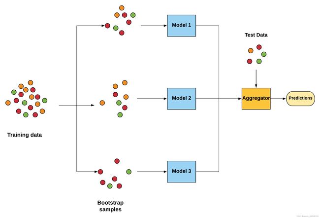
集成学习（ensemble learning），并不是一个单独的机器学习算法，而是通过构建并结合多个机器学习器（基学习器，Base learner）来完成学习任务。
对于训练集数据，我们通过训练若干个个体弱学习器（weak learner），通过一定的结合策略，就可以最终形成一个强学习器（strong learner），以达到博采众长的目的。

我们首先将建立一个随机森林模型，这是一个称为Bagging类型的集成类型算法。这个模型由几个“树”组成（我们将构造100棵树！）这将独立考虑每对新闻标题的LSI向量数据，可以并行运行。然后，随机森林模型做出一个民主决策，投票决定属于哪种分类关系。

我们使用 scikit-learn 中的 RandomForestClassifier 函数实现随机森林模型。

之后我们再建立一个梯度提升树模型，它属于所谓Boosting系列算法。多个学习器是依次构建的，个体学习器之间存在强依赖关系，需要串行生成。

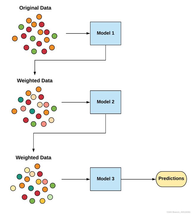
我们使用 scikit-learn 中的 GradientBoostingClassifier 函数实现梯度提升树模型。

# Random Forest Classifier 
 
from sklearn.ensemble import RandomForestClassifier 
 
rfc = RandomForestClassifier(n_estimators=100, max_depth=5, random_state=1) 
rfc.fit(x_train, y_train) 
 
predictions = rfc.predict(x_val) 
predictions 

array([0, 0, 1, ..., 0, 0, 0], dtype=int64)

我们可以直接调用 scikit-learn 中的 accuracy_score 函数计算这个随机森林模型在验证集上的准确率。

from sklearn.metrics import accuracy_score 
 
# acc_rfc = round(accuracy_score(predictions, np.eye(3)[y_val]) * 100, 2) 
acc_rfc = round(accuracy_score(predictions, y_val) * 100, 2) 
print('Accurency of RandomForestClassifier: {:.1f}%'.format(acc_rfc)) 

Accurency of RandomForestClassifier: 71.5%

# Gradient Boosting Classifier 
from sklearn.ensemble import GradientBoostingClassifier 
 
gbk = GradientBoostingClassifier() 
gbk.fit(x_train, y_train) 
y_pred = gbk.predict(x_val) 
acc_gbk = round(accuracy_score(y_pred, y_val) * 100, 2) 
print('Accurency of GradientBoostingClassifier: {:.1f}%'.format(acc_gbk)) 

Accurency of GradientBoostingClassifier: 73.0%

效果比较好的是梯度提升树模型，准确率的结果是73.0%，与通过简单的LSI向量余弦距离方法仅有很微弱的提升，这可能是LSI数据供给的能力上限了。

之后，我们将从一个全新的视角来处理文档的数字化表示，力求保留下更完整的数据信息供模型所用。

---

好了，就到这儿吧。

本系列共12期，将分6天发布。相关代码已全部分享在我的github项目（moronism189/chinese-nlp-stepbystep）下，急的可以先去那里下载。