用Keras构建AutoEncoder

用Keras构建AutoEncoder

原文链接：Building Autoencoders in Keras
在本教程中，我们将回答一些关于自动编码器的常见问题，并将介绍以下模型的代码示例：

• 一个基于全连接层的简单自动编码器
• 一个稀疏自动编码器
• 一个深度全连接的自动编码器
• 一种图像去噪模型
• 一个sequence-to-sequence的自动编码器
• 一个变分自动编码器（VAE）

注:所有代码示例已于2017年3月14日更新到Keras 2.0 API。您将需要Keras版本2.0.0或更高版本来运行它们。

什么是自动编码器

“自动编码”是一种数据压缩算法，其中的压缩和解压缩函数是1）特定于数据的，2）有损的，3）从例子中自动学习而不是人工设计的。此外，几乎在所有使用术语“自动编码器”的上下文中，压缩和解压缩函数都是用神经网络实现的。

1. 自动编码器是特定于数据的，这意味着他们只能压缩类似于他们所训练的数据。这与MPEG-2 Audio Layer III (MP3)压缩算法不同，后者只对“声音”进行一般假设，而不需要是特定类型的声音。对人脸图片进行训练的自动编码器在压缩树木图片方面做得相当差，因为它将学到的特征是特定于人脸的。
2. 自动编码器是有损的，这意味着与原始输入(类似于MP3或JPEG压缩)相比，解压后的输出将会降级。这与无损算术压缩不同。
3. 自动编码器是通过数据示例自动学习的，这是一个有用的特性：它意味着很容易训练算法的特定实例，使其在特定类型的输入上表现良好。它不需要任何新的编码，只需要适当的训练数据。

要构建一个自动编码器，您需要三样东西：一个编码函数、一个解码函数，以及数据的压缩表示与解压缩表示之间的信息丢失量之间的距离函数（即“损失”函数）。编码器和解码器将被选择为参数函数(通常是神经网络)，并且相对于距离函数是可微的，因此可以使用随机梯度下降对编码/解码函数的参数进行优化，以最小化重构损失。很简单!你甚至不需要理解这些单词就可以在实践中开始使用自动编码器。

他们擅长数据压缩吗?

通常，不是真的。例如在图像压缩方面，很难训练出一个比JPEG等基本算法做的更好的自动编码器。通常实现它的唯一方法就是通过限制自己在一个非常特定类型的图片（比如在这个方面JPEG做的不好）。事实上，自动编码器是特定于数据的，这使得它们通常不适用于实际的数据压缩问题:您只能在与它们所训练的内容类似的数据上使用它们，因此使它们更通用需要大量的训练数据。但未来的进步可能会改变这一点，谁知道呢。

自动编码器擅长做什么?

它们很少在实际应用中使用。2012年，他们在深度卷积神经网络[1]的贪婪分层预训练中发现了一个应用，但当我们开始意识到更好的随机权重初始化方案足以从头开始训练深度网络时，这种方法很快就过时了。2014年，批处理标准化[2]开始允许更深层的网络，从2015年末开始，我们可以使用残差学习[3]从零开始训练任意深度的网络。

今天，自动编码器的两个有趣的实际应用是数据去噪（我们将在本文后面介绍）和数据可视化的降维。通过适当的维数和稀疏性约束，自动编码器可以学习比PCA或其他基本技术更有趣的数据投影。

对于二维可视化，t-SNE(发音为“tee-snee”)可能是最好的算法，但它通常需要相对低维的数据。因此，在高维数据中可视化相似性关系的一个好策略是，首先使用自动编码器将数据压缩到低维空间（例如32维），然后使用t-SNE将压缩数据映射到二维平面。注意，Keras中一个很好的参数化t-SNE实现是由Kyle McDonald开发的，可以在Github上使用。另外，scikit-learn也有一个简单而实用的实现。

那自动编码器有什么大的用处呢？

他们成名的主要原因是在网上许多介绍性的机器学习课程中都有介绍。因此，这个领域的许多新来者都非常喜欢自动编码器，而且这些对他们还不够。这就是本教程存在的原因！
否则，它们吸引如此多的研究和关注的一个原因是，长期以来，它们一直被认为是解决无监督学习问题的潜在途径，例如学习有用的表示而不需要标签。然而，自动编码器并不是一种真正的无监督学习技术（这意味着完全不同的学习过程），而是一种自我监督的技术，是监督学习的一个特定实例，目标是由输入数据生成的。为了让自我监督的模型学习有趣的特性，你必须想出一个有趣的合成目标和损失函数，这就是问题的所在：仅仅学习重新构建输入的微小细节可能不是正确的选择。在这一点上有显著的证据表明，专注于重建一幅在像素级别，例如，不利于学习有趣，那种label-supervized学习引发的抽象特性(在目标相当抽象概念等人类“发明”的“狗”,“车”…)。事实上，有人可能会说，在这方面最好的特性是那些在精确输入重建方面最差的特性，同时在您感兴趣的主要任务(分类、定位等)上获得高性能。自监督学习应用于计算机视觉，一个潜在的富有成效的自编码类型的输入重建的选择是用于玩具任务，例如解决拼图游戏问题，或详细上下文匹配（能够匹配高分辨率，以及从高分辨率图片抽取的低分辨率版本的小片图片）。下面这篇文章研究了拼图游戏的解法，读起来很有趣：Noroozi and Favaro (2016) Unsupervised Learning of Visual Representations by Solving Jigsaw Puzzles。这些任务为模型提供了关于输入数据的内置假设，而这些假设是传统自动编码器所缺少的，比如“视觉宏观结构比像素级细节更重要”。

让我们来构建可能是最简单的自动编码器

我们将从简单的开始，一个单一的完全连接的神经层作为编码器和解码器：

from keras.layers import Input, Dense
from keras.models import Model

# this is the size of our encoded representations
encoding_dim = 32  # 32 floats -> compression of factor 24.5, assuming the input is 784 floats

# this is our input placeholder
input_img = Input(shape=(784,))
# "encoded" is the encoded representation of the input
encoded = Dense(encoding_dim, activation='relu')(input_img)
# "decoded" is the lossy reconstruction of the input
decoded = Dense(784, activation='sigmoid')(encoded)

# this model maps an input to its reconstruction
autoencoder = Model(input_img, decoded)

让我们也创建一个单独的编码器模型：

# this model maps an input to its encoded representation
encoder = Model(input_img, encoded)

以及解码器模型：

# create a placeholder for an encoded (32-dimensional) input
encoded_input = Input(shape=(encoding_dim,))
# retrieve the last layer of the autoencoder model
decoder_layer = autoencoder.layers[-1]
# create the decoder model
decoder = Model(encoded_input, decoder_layer(encoded_input))

现在让我们训练我们的自动编码器来重建MNIST数字。

首先，我们将配置我们的模型使用每像素的二分类交叉熵损失，和Adadelta优化器:

autoencoder.compile(optimizer='adadelta', loss='binary_crossentropy')

让我们准备输入数据。我们将使用MNIST数字，并丢弃标签（因为我们只对编码/解码输入图像感兴趣）。

from keras.datasets import mnist
import numpy as np
(x_train, _), (x_test, _) = mnist.load_data()

我们将对0到1之间的所有值进行标准化，并将28x28张图像压平为大小为784的向量。

x_train = x_train.astype('float32') / 255.
x_test = x_test.astype('float32') / 255.
x_train = x_train.reshape((len(x_train), np.prod(x_train.shape[1:])))
x_test = x_test.reshape((len(x_test), np.prod(x_test.shape[1:])))
print x_train.shape
print x_test.shape

现在让我们训练我们的自动编码器50个周期：

autoencoder.fit(x_train, x_train,
                epochs=50,
                batch_size=256,
                shuffle=True,
                validation_data=(x_test, x_test))

经过50个周期后，自动编码器似乎达到了一个稳定的训练/测试损失值约0.11。我们可以尝试可视化重建的输入和编码的表示。我们将使用Matplotlib。

# encode and decode some digits
# note that we take them from the *test* set
encoded_imgs = encoder.predict(x_test)
decoded_imgs = decoder.predict(encoded_imgs)

# use Matplotlib (don't ask)
import matplotlib.pyplot as plt

n = 10  # how many digits we will display
plt.figure(figsize=(20, 4))
for i in range(n):
    # display original
    ax = plt.subplot(2, n, i + 1)
    plt.imshow(x_test[i].reshape(28, 28))
    plt.gray()
    ax.get_xaxis().set_visible(False)
    ax.get_yaxis().set_visible(False)

    # display reconstruction
    ax = plt.subplot(2, n, i + 1 + n)
    plt.imshow(decoded_imgs[i].reshape(28, 28))
    plt.gray()
    ax.get_xaxis().set_visible(False)
    ax.get_yaxis().set_visible(False)
plt.show()

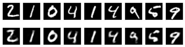
这是我们得到的。上面一行是原始数字，下面一行是重建后的数字。使用这种基本方法，我们正在丢失相当多的细节。

在编码表示上添加稀疏约束

在前面的例子中，表示只受隐藏层大小的限制（32）。在这种情况下，通常发生的是隐含层正在学习PCA(主成分分析)的近似。但是约束表示为紧凑的另一种方法是对隐藏表示的活动添加稀疏约束，这样在给定的时间内会“触发”更少的单元。在Keras中，这可以通过添加activity_regularizer到我们的Dense层来实现：

from keras import regularizers

encoding_dim = 32

input_img = Input(shape=(784,))
# add a Dense layer with a L1 activity regularizer
encoded = Dense(encoding_dim, activation='relu',
                activity_regularizer=regularizers.l1(10e-5))(input_img)
decoded = Dense(784, activation='sigmoid')(encoded)

autoencoder = Model(input_img, decoded)

让我们对这个模型进行100个周期的训练（加上正则化，该模型不太可能过度拟合，并且可以训练更长时间）。模型以0.11的训练损失和0.10的测试损失结束。两者之间的差异主要是在训练过程中在损失中增加了正则化项（值约值0.01）。
以下是我们的新结果的可视化：

它们看起来与之前的模型非常相似，唯一显著的区别是编码表示的稀疏性。encoded_imgs.mean()的值为3.33(在10,000个测试图像上)，而前一个模型的值为7.30。因此，我们的新模型产生了两倍稀疏的编码表示。

深度自编码器

我们不需要把自己限制在用一个单一的层作为编码器或解码器，我们可以使用一堆层，如：

input_img = Input(shape=(784,))
encoded = Dense(128, activation='relu')(input_img)
encoded = Dense(64, activation='relu')(encoded)
encoded = Dense(32, activation='relu')(encoded)

decoded = Dense(64, activation='relu')(encoded)
decoded = Dense(128, activation='relu')(decoded)
decoded = Dense(784, activation='sigmoid')(decoded)

让我们试试这个：

autoencoder = Model(input_img, decoded)
autoencoder.compile(optimizer='adadelta', loss='binary_crossentropy')

autoencoder.fit(x_train, x_train,
                epochs=100,
                batch_size=256,
                shuffle=True,
                validation_data=(x_test, x_test))

经过100个周期后，达到训练和测试损失约为0.097，略好于我们之前的模型。我们重建的数字看起来也更好：

卷积自编码器

由于我们的输入是图像，因此使用卷积神经网络(convnets)作为编码器和解码器是有意义的。在实际环境中，应用于图像的自动编码器通常是卷积式自动编码器——它们的性能要好得多。
让我们实现一个。编码器将由一堆的Conv2D层和MaxPooling2D层(最大池化层用于空间下采样)组成，而解码器将由一堆的Conv2D和UpSampling2D层组成。

from keras.layers import Input, Dense, Conv2D, MaxPooling2D, UpSampling2D
from keras.models import Model
from keras import backend as K

input_img = Input(shape=(28, 28, 1))  # adapt this if using `channels_first` image data format

x = Conv2D(16, (3, 3), activation='relu', padding='same')(input_img)
x = MaxPooling2D((2, 2), padding='same')(x)
x = Conv2D(8, (3, 3), activation='relu', padding='same')(x)
x = MaxPooling2D((2, 2), padding='same')(x)
x = Conv2D(8, (3, 3), activation='relu', padding='same')(x)
encoded = MaxPooling2D((2, 2), padding='same')(x)

# at this point the representation is (4, 4, 8) i.e. 128-dimensional

x = Conv2D(8, (3, 3), activation='relu', padding='same')(encoded)
x = UpSampling2D((2, 2))(x)
x = Conv2D(8, (3, 3), activation='relu', padding='same')(x)
x = UpSampling2D((2, 2))(x)
x = Conv2D(16, (3, 3), activation='relu')(x)
x = UpSampling2D((2, 2))(x)
decoded = Conv2D(1, (3, 3), activation='sigmoid', padding='same')(x)

autoencoder = Model(input_img, decoded)
autoencoder.compile(optimizer='adadelta', loss='binary_crossentropy')

为了训练它，我们将使用原始MNIST数字的形状(samples,3,28,28)，我们只是将像素值标准化为0和1之间的值。

from keras.datasets import mnist
import numpy as np

(x_train, _), (x_test, _) = mnist.load_data()

x_train = x_train.astype('float32') / 255.
x_test = x_test.astype('float32') / 255.
x_train = np.reshape(x_train, (len(x_train), 28, 28, 1))  # adapt this if using `channels_first` image data format
x_test = np.reshape(x_test, (len(x_test), 28, 28, 1))  # adapt this if using `channels_first` image data format

让我们把这个模型训练50个周期。为了演示如何在训练期间可视化模型的结果，我们将使用TensorFlow后端和TensorBoard回调函数。

首先，让我们打开一个终端并启动一个TensorBoard服务器，它将读取存储在/tmp/autoencoder中的日志。

tensorboard --logdir=/tmp/autoencoder

然后我们来训练我们的模型。在callbacks列表中，我们传递一个TensorBoard回调的实例。在每个周期之后，这个回调函数将向/tmp/autoencoder写入日志，我们的TensorBoard服务器可以读取这些日志。

from keras.callbacks import TensorBoard

autoencoder.fit(x_train, x_train,
                epochs=50,
                batch_size=128,
                shuffle=True,
                validation_data=(x_test, x_test),
                callbacks=[TensorBoard(log_dir='/tmp/autoencoder')])

这允许我们再TensorBoard网络接口上监控训练（通过访问http://0.0.0.0:6006）

该模型收敛到0.094的损失，显著优于我们之前的模型(这在很大程度上是由于编码表示的更高的熵容量，128维与之前的32维相比)。让我们来看看重建的数字：

decoded_imgs = autoencoder.predict(x_test)

n = 10
plt.figure(figsize=(20, 4))
for i in range(n):
    # display original
    ax = plt.subplot(2, n, i)
    plt.imshow(x_test[i].reshape(28, 28))
    plt.gray()
    ax.get_xaxis().set_visible(False)
    ax.get_yaxis().set_visible(False)

    # display reconstruction
    ax = plt.subplot(2, n, i + n)
    plt.imshow(decoded_imgs[i].reshape(28, 28))
    plt.gray()
    ax.get_xaxis().set_visible(False)
    ax.get_yaxis().set_visible(False)
plt.show()

我们还可以看看128维编码表示。这些表示形式是8x4x4，因此我们将它们重新塑造为4x32，以便能够将它们显示为灰度图像。

n = 10
plt.figure(figsize=(20, 8))
for i in range(n):
    ax = plt.subplot(1, n, i)
    plt.imshow(encoded_imgs[i].reshape(4, 4 * 8).T)
    plt.gray()
    ax.get_xaxis().set_visible(False)
    ax.get_yaxis().set_visible(False)
plt.show()

应用于图像去噪

让我们用卷积自编码器来处理一个图像去噪问题。这很简单：我们将训练自动编码器映射有噪声的数字图像到干净的数字图像。
这是我们将会如何生成合并噪声的数字：我们只是应用一个高斯噪声矩阵，并剪辑图像使它的值在0和1之间。

from keras.datasets import mnist
import numpy as np

(x_train, _), (x_test, _) = mnist.load_data()

x_train = x_train.astype('float32') / 255.
x_test = x_test.astype('float32') / 255.
x_train = np.reshape(x_train, (len(x_train), 28, 28, 1))  # adapt this if using `channels_first` image data format
x_test = np.reshape(x_test, (len(x_test), 28, 28, 1))  # adapt this if using `channels_first` image data format

noise_factor = 0.5
x_train_noisy = x_train + noise_factor * np.random.normal(loc=0.0, scale=1.0, size=x_train.shape) 
x_test_noisy = x_test + noise_factor * np.random.normal(loc=0.0, scale=1.0, size=x_test.shape) 

x_train_noisy = np.clip(x_train_noisy, 0., 1.)
x_test_noisy = np.clip(x_test_noisy, 0., 1.)

下面是这些带噪音的数字的样子：

n = 10
plt.figure(figsize=(20, 2))
for i in range(n):
    ax = plt.subplot(1, n, i)
    plt.imshow(x_test_noisy[i].reshape(28, 28))
    plt.gray()
    ax.get_xaxis().set_visible(False)
    ax.get_yaxis().set_visible(False)
plt.show()

如果你眯着眼睛，你仍然能认出他们，但几乎认不出来。我们的自动编码器能学会恢复原始数字吗?让我们找出答案。
与之前的卷积自编码器相比，为了提高重建的质量，我们将使用稍微不同的模型，每层有更多的过滤器：

input_img = Input(shape=(28, 28, 1))  # adapt this if using `channels_first` image data format

x = Conv2D(32, (3, 3), activation='relu', padding='same')(input_img)
x = MaxPooling2D((2, 2), padding='same')(x)
x = Conv2D(32, (3, 3), activation='relu', padding='same')(x)
encoded = MaxPooling2D((2, 2), padding='same')(x)

# at this point the representation is (7, 7, 32)

x = Conv2D(32, (3, 3), activation='relu', padding='same')(encoded)
x = UpSampling2D((2, 2))(x)
x = Conv2D(32, (3, 3), activation='relu', padding='same')(x)
x = UpSampling2D((2, 2))(x)
decoded = Conv2D(1, (3, 3), activation='sigmoid', padding='same')(x)

autoencoder = Model(input_img, decoded)
autoencoder.compile(optimizer='adadelta', loss='binary_crossentropy')

让我们来训练这个模型100个周期：

autoencoder.fit(x_train_noisy, x_train,
                epochs=100,
                batch_size=128,
                shuffle=True,
                validation_data=(x_test_noisy, x_test),
                callbacks=[TensorBoard(log_dir='/tmp/tb', histogram_freq=0, write_graph=False)])

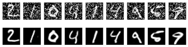
现在让我们看看结果。顶部是输入到网络的噪声数字，底部是由网络重构的数字。

看起来效果不错。如果将此过程扩展到更大的convnet，则可以开始构建文档降噪或音频降噪模型。Kaggle有一个有趣的数据集可以帮助您入门。

Sequence-to-sequence 自编码器

如果您输入的是序列，而不是向量或2D图像，那么您可能想要使用一种能够捕获时间结构的模型作为编码器和解码器，比如LSTM。为了建立一个基于LSTM的自编码器，首先使用一个LSTM编码器将输入序列转换为一个包含整个序列信息的单一向量，然后重复这个向量n次（其中n是输出序列中的时间步长），然后运行一个LSTM解码器将这个常数序列转换为目标序列。
我们不会在任何特定的数据集上演示它。我们将在这里放一个代码示例供读者参考！

from keras.layers import Input, LSTM, RepeatVector
from keras.models import Model

inputs = Input(shape=(timesteps, input_dim))
encoded = LSTM(latent_dim)(inputs)

decoded = RepeatVector(timesteps)(encoded)
decoded = LSTM(input_dim, return_sequences=True)(decoded)

sequence_autoencoder = Model(inputs, decoded)
encoder = Model(inputs, encoded)

变分自编码器（VAE）

变分自编码器是一种更现代、更有趣的自编码方式。
你可能会问，什么是变分自动编码器？它是一种自动编码器，对正在学习的编码表示形式添加了约束。更准确地说，它是一个自动编码器，为其输入数据学习一个潜在变量模型。所以不是让你的神经网络学习任意函数，而是学习概率分布的参数来建模你的数据。如果从这个分布中采样点，就可以生成新的输入数据样本：VAE是一个“生成模型”。
变分自动编码器是如何工作的？
首先，编码器网络将输入样本x转换为潜在空间中的两个参数，我们将记为z_mean和z_log_sigma。然后，我们通过$z=z\_mean+exp(z\_log\_sigma)\ast epsilon$，从假设用于生成数据的潜在正态分布中随机抽取相似点z，其中$epsilon$为随机正态张量。最后，解码器网络将这些潜在空间点映射回原始输入数据。
模型的参数通过两个损失函数进行训练：重构损失迫使解码后的样本与初始输入匹配（就像我们之前的自动编码器一样），以及学习到的潜在分布与先验分布之间的KL散度，作为正则项。实际上，您可以完全摆脱后一项，尽管它确实有助于学习格式良好的潜在空间和减少对训练数据的过度拟合。
因为VAE是一个更复杂的示例，所以我们将代码作为独立的脚本放在Github上。在这里，我们将逐步回顾模型是如何创建的。
首先，这是我们的编码器网络，将输入映射到潜在的分布参数：

x = Input(batch_shape=(batch_size, original_dim))
h = Dense(intermediate_dim, activation='relu')(x)
z_mean = Dense(latent_dim)(h)
z_log_sigma = Dense(latent_dim)(h)

我们可以利用这些参数从潜在空间中采样新的相似点：

def sampling(args):
    z_mean, z_log_sigma = args
    epsilon = K.random_normal(shape=(batch_size, latent_dim),
                              mean=0., std=epsilon_std)
    return z_mean + K.exp(z_log_sigma) * epsilon

# note that "output_shape" isn't necessary with the TensorFlow backend
# so you could write `Lambda(sampling)([z_mean, z_log_sigma])`
z = Lambda(sampling, output_shape=(latent_dim,))([z_mean, z_log_sigma])

最后，我们可以将这些采样的潜在点映射回重构的输入：

decoder_h = Dense(intermediate_dim, activation='relu')
decoder_mean = Dense(original_dim, activation='sigmoid')
h_decoded = decoder_h(z)
x_decoded_mean = decoder_mean(h_decoded)

到目前为止，我们所做的让我们可以实例化3个模型：

• 一个用于将输入映射到重构的端到端的自动编码器
• 一个编码器用于将输入映射到潜在空间
• 一个能从潜在空间获取点，并输出对应的重建样本的生成器

# end-to-end autoencoder
vae = Model(x, x_decoded_mean)

# encoder, from inputs to latent space
encoder = Model(x, z_mean)

# generator, from latent space to reconstructed inputs
decoder_input = Input(shape=(latent_dim,))
_h_decoded = decoder_h(decoder_input)
_x_decoded_mean = decoder_mean(_h_decoded)
generator = Model(decoder_input, _x_decoded_mean)

我们使用端到端模型训练模型，使用自定义损失函数:重建项和KL散度正则化项的和。

def vae_loss(x, x_decoded_mean):
    xent_loss = objectives.binary_crossentropy(x, x_decoded_mean)
    kl_loss = - 0.5 * K.mean(1 + z_log_sigma - K.square(z_mean) - K.exp(z_log_sigma), axis=-1)
    return xent_loss + kl_loss

vae.compile(optimizer='rmsprop', loss=vae_loss)

我们在MNIST数字上训练VAE：

(x_train, y_train), (x_test, y_test) = mnist.load_data()

x_train = x_train.astype('float32') / 255.
x_test = x_test.astype('float32') / 255.
x_train = x_train.reshape((len(x_train), np.prod(x_train.shape[1:])))
x_test = x_test.reshape((len(x_test), np.prod(x_test.shape[1:])))

vae.fit(x_train, x_train,
        shuffle=True,
        epochs=epochs,
        batch_size=batch_size,
        validation_data=(x_test, x_test))

因为我们的潜在空间是二维的，所以在这一点上可以做一些很酷的可视化。一是在潜在的二维平面上观察不同类别的邻域：

x_test_encoded = encoder.predict(x_test, batch_size=batch_size)
plt.figure(figsize=(6, 6))
plt.scatter(x_test_encoded[:, 0], x_test_encoded[:, 1], c=y_test)
plt.colorbar()
plt.show()

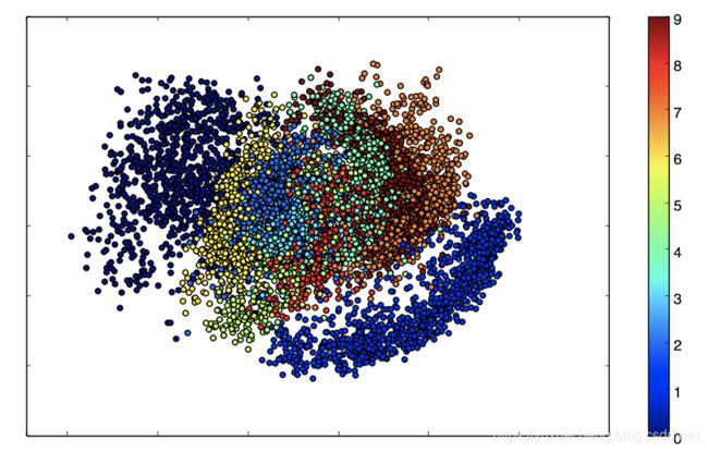
这些彩色的集群中的每一种颜色都是一种类型的数字。紧密集群是结构相似的数字（即在潜在空间中共享信息的数字）。
因为VAE是一个生成模型，我们也可以使用它来生成新的数字！在这里，我们将扫描潜在平面，定期采样潜在点，并为每个点生成对应的数字。这让我们看到了“生成”MNIST数字的潜在多样性。

# display a 2D manifold of the digits
n = 15  # figure with 15x15 digits
digit_size = 28
figure = np.zeros((digit_size * n, digit_size * n))
# we will sample n points within [-15, 15] standard deviations
grid_x = np.linspace(-15, 15, n)
grid_y = np.linspace(-15, 15, n)

for i, yi in enumerate(grid_x):
    for j, xi in enumerate(grid_y):
        z_sample = np.array([[xi, yi]]) * epsilon_std
        x_decoded = generator.predict(z_sample)
        digit = x_decoded[0].reshape(digit_size, digit_size)
        figure[i * digit_size: (i + 1) * digit_size,
               j * digit_size: (j + 1) * digit_size] = digit

plt.figure(figsize=(10, 10))
plt.imshow(figure)
plt.show()

就是这样！如果您对本文（或以后的文章）中涉及的更多主题有任何建议，请通过Twitter @fchollet与我联系。

参考文献

References

[1] Why does unsupervised pre-training help deep learning?

[2] Batch normalization: Accelerating deep network training by reducing internal covariate shift.

[3] Deep Residual Learning for Image Recognition

[4] Auto-Encoding Variational Bayes