- 机器学习与深度学习间关系与区别
ℒℴѵℯ心·动ꦿ໊ོ꫞
人工智能学习深度学习python
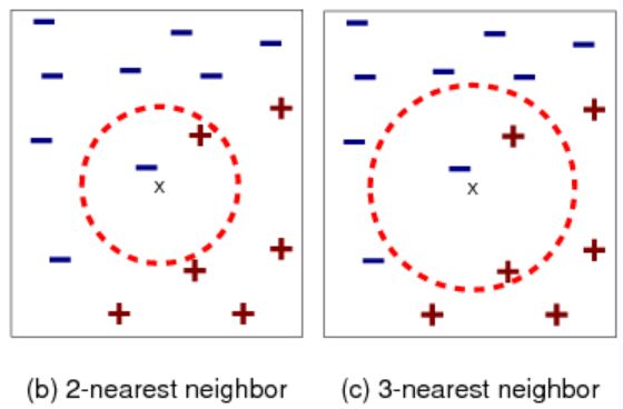
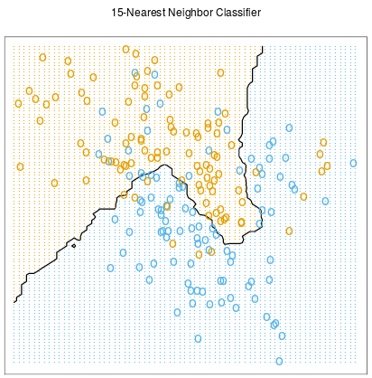
一、机器学习概述定义机器学习(MachineLearning,ML)是一种通过数据驱动的方法,利用统计学和计算算法来训练模型,使计算机能够从数据中学习并自动进行预测或决策。机器学习通过分析大量数据样本,识别其中的模式和规律,从而对新的数据进行判断。其核心在于通过训练过程,让模型不断优化和提升其预测准确性。主要类型1.监督学习(SupervisedLearning)监督学习是指在训练数据集中包含输入
- 理解Gunicorn:Python WSGI服务器的基石
范范0825
ipythonlinux运维
理解Gunicorn:PythonWSGI服务器的基石介绍Gunicorn,全称GreenUnicorn,是一个为PythonWSGI(WebServerGatewayInterface)应用设计的高效、轻量级HTTP服务器。作为PythonWeb应用部署的常用工具,Gunicorn以其高性能和易用性著称。本文将介绍Gunicorn的基本概念、安装和配置,帮助初学者快速上手。1.什么是Gunico
- Python数据分析与可视化实战指南
William数据分析
pythonpython数据
在数据驱动的时代,Python因其简洁的语法、强大的库生态系统以及活跃的社区,成为了数据分析与可视化的首选语言。本文将通过一个详细的案例,带领大家学习如何使用Python进行数据分析,并通过可视化来直观呈现分析结果。一、环境准备1.1安装必要库在开始数据分析和可视化之前,我们需要安装一些常用的库。主要包括pandas、numpy、matplotlib和seaborn等。这些库分别用于数据处理、数学
- python os.environ
江湖偌大
python深度学习
os.environ['TF_CPP_MIN_LOG_LEVEL']='0'#默认值,输出所有信息os.environ['TF_CPP_MIN_LOG_LEVEL']='1'#屏蔽通知信息(INFO)os.environ['TF_CPP_MIN_LOG_LEVEL']='2'#屏蔽通知信息和警告信息(INFO\WARNING)os.environ['TF_CPP_MIN_LOG_LEVEL']='
- Python中os.environ基本介绍及使用方法
鹤冲天Pro
#Pythonpython服务器开发语言
文章目录python中os.environos.environ简介os.environ进行环境变量的增删改查python中os.environ的使用详解1.简介2.key字段详解2.1常见key字段3.os.environ.get()用法4.环境变量的增删改查和判断是否存在4.1新增环境变量4.2更新环境变量4.3获取环境变量4.4删除环境变量4.5判断环境变量是否存在python中os.envi
- Pyecharts数据可视化大屏:打造沉浸式数据分析体验
我的运维人生
信息可视化数据分析数据挖掘运维开发技术共享
Pyecharts数据可视化大屏:打造沉浸式数据分析体验在当今这个数据驱动的时代,如何将海量数据以直观、生动的方式展现出来,成为了数据分析师和企业决策者关注的焦点。Pyecharts,作为一款基于Python的开源数据可视化库,凭借其丰富的图表类型、灵活的配置选项以及高度的定制化能力,成为了构建数据可视化大屏的理想选择。本文将深入探讨如何利用Pyecharts打造数据可视化大屏,并通过实际代码案例
- Goolge earth studio 进阶4——路径修改与平滑
陟彼高冈yu
Googleearthstudio进阶教程旅游
如果我们希望在大约中途时获得更多的城市鸟瞰视角。可以将相机拖动到这里并创建一个新的关键帧。camera_target_clip_7EarthStudio会自动平滑我们的路径,所以当我们通过这个关键帧时,不是一个生硬的角度,而是一个平滑的曲线。camera_target_clip_8路径上有贝塞尔控制手柄,允许我们调整路径的形状。右键单击,我们可以选择“平滑路径”,这是默认的自动平滑算法,或者我们可
- Python教程:一文了解使用Python处理XPath
旦莫
Python进阶python开发语言
目录1.环境准备1.1安装lxml1.2验证安装2.XPath基础2.1什么是XPath?2.2XPath语法2.3示例XML文档3.使用lxml解析XML3.1解析XML文档3.2查看解析结果4.XPath查询4.1基本路径查询4.2使用属性查询4.3查询多个节点5.XPath的高级用法5.1使用逻辑运算符5.2使用函数6.实战案例6.1从网页抓取数据6.1.1安装Requests库6.1.2代
- python os.environ_python os.environ 读取和设置环境变量
weixin_39605414
pythonos.environ
>>>importos>>>os.environ.keys()['LC_NUMERIC','GOPATH','GOROOT','GOBIN','LESSOPEN','SSH_CLIENT','LOGNAME','USER','HOME','LC_PAPER','PATH','DISPLAY','LANG','TERM','SHELL','J2REDIR','LC_MONETARY','QT_QPA
- 基于社交网络算法优化的二维最大熵图像分割
智能算法研学社(Jack旭)
智能优化算法应用图像分割算法php开发语言
智能优化算法应用:基于社交网络优化的二维最大熵图像阈值分割-附代码文章目录智能优化算法应用:基于社交网络优化的二维最大熵图像阈值分割-附代码1.前言2.二维最大熵阈值分割原理3.基于社交网络优化的多阈值分割4.算法结果:5.参考文献:6.Matlab代码摘要:本文介绍基于最大熵的图像分割,并且应用社交网络算法进行阈值寻优。1.前言阅读此文章前,请阅读《图像分割:直方图区域划分及信息统计介绍》htt
- 探索OpenAI和LangChain的适配器集成:轻松切换模型提供商
nseejrukjhad
langchaineasyui前端python
#探索OpenAI和LangChain的适配器集成:轻松切换模型提供商##引言在人工智能和自然语言处理的世界中,OpenAI的模型提供了强大的能力。然而,随着技术的发展,许多人开始探索其他模型以满足特定需求。LangChain作为一个强大的工具,集成了多种模型提供商,通过提供适配器,简化了不同模型之间的转换。本篇文章将介绍如何使用LangChain的适配器与OpenAI集成,以便轻松切换模型提供商
- 使用Faiss进行高效相似度搜索
llzwxh888
faisspython
在现代AI应用中,快速和高效的相似度搜索是至关重要的。Faiss(FacebookAISimilaritySearch)是一个专门用于快速相似度搜索和聚类的库,特别适用于高维向量。本文将介绍如何使用Faiss来进行相似度搜索,并结合Python代码演示其基本用法。什么是Faiss?Faiss是一个由FacebookAIResearch团队开发的开源库,主要用于高维向量的相似性搜索和聚类。Faiss
- python是什么意思中文-在python中%是什么意思
编程大乐趣
Python中%有两种:1、数值运算:%代表取模,返回除法的余数。如:>>>7%212、%操作符(字符串格式化,stringformatting),说明如下:%[(name)][flags][width].[precision]typecode(name)为命名flags可以有+,-,''或0。+表示右对齐。-表示左对齐。''为一个空格,表示在正数的左侧填充一个空格,从而与负数对齐。0表示使用0填
- 深入理解 MultiQueryRetriever:提升向量数据库检索效果的强大工具
nseejrukjhad
数据库python
深入理解MultiQueryRetriever:提升向量数据库检索效果的强大工具引言在人工智能和自然语言处理领域,高效准确的信息检索一直是一个关键挑战。传统的基于距离的向量数据库检索方法虽然广泛应用,但仍存在一些局限性。本文将介绍一种创新的解决方案:MultiQueryRetriever,它通过自动生成多个查询视角来增强检索效果,提高结果的相关性和多样性。MultiQueryRetriever的工
- Day1笔记-Python简介&标识符和关键字&输入输出
~在杰难逃~
Pythonpython开发语言大数据数据分析数据挖掘
大家好,从今天开始呢,杰哥开展一个新的专栏,当然,数据分析部分也会不定时更新的,这个新的专栏主要是讲解一些Python的基础语法和知识,帮助0基础的小伙伴入门和学习Python,感兴趣的小伙伴可以开始认真学习啦!一、Python简介【了解】1.计算机工作原理编程语言就是用来定义计算机程序的形式语言。我们通过编程语言来编写程序代码,再通过语言处理程序执行向计算机发送指令,让计算机完成对应的工作,编程
- python八股文面试题分享及解析(1)
Shawn________
python
#1.'''a=1b=2不用中间变量交换a和b'''#1.a=1b=2a,b=b,aprint(a)print(b)结果:21#2.ll=[]foriinrange(3):ll.append({'num':i})print(11)结果:#[{'num':0},{'num':1},{'num':2}]#3.kk=[]a={'num':0}foriinrange(3):#0,12#可变类型,不仅仅改变
- 121. 买卖股票的最佳时机
薄荷糖的味道_fb40
给定一个数组,它的第i个元素是一支给定股票第i天的价格。如果你最多只允许完成一笔交易(即买入和卖出一支股票),设计一个算法来计算你所能获取的最大利润。注意你不能在买入股票前卖出股票。示例1:输入:[7,1,5,3,6,4]输出:5解释:在第2天(股票价格=1)的时候买入,在第5天(股票价格=6)的时候卖出,最大利润=6-1=5。注意利润不能是7-1=6,因为卖出价格需要大于买入价格。示例2:输入:
- 人工智能时代,程序员如何保持核心竞争力?
jmoych
人工智能
随着AIGC(如chatgpt、midjourney、claude等)大语言模型接二连三的涌现,AI辅助编程工具日益普及,程序员的工作方式正在发生深刻变革。有人担心AI可能取代部分编程工作,也有人认为AI是提高效率的得力助手。面对这一趋势,程序员应该如何应对?是专注于某个领域深耕细作,还是广泛学习以适应快速变化的技术环境?又或者,我们是否应该将重点转向AI无法轻易替代的软技能?让我们一起探讨程序员
- 每日算法&面试题,大厂特训二十八天——第二十天(树)
肥学
⚡算法题⚡面试题每日精进java算法数据结构
目录标题导读算法特训二十八天面试题点击直接资料领取导读肥友们为了更好的去帮助新同学适应算法和面试题,最近我们开始进行专项突击一步一步来。上一期我们完成了动态规划二十一天现在我们进行下一项对各类算法进行二十八天的一个小总结。还在等什么快来一起肥学进行二十八天挑战吧!!特别介绍小白练手专栏,适合刚入手的新人欢迎订阅编程小白进阶python有趣练手项目里面包括了像《机器人尬聊》《恶搞程序》这样的有趣文章
- Python快速入门 —— 第三节:类与对象
孤华暗香
Python快速入门python开发语言
第三节:类与对象目标:了解面向对象编程的基础概念,并学会如何定义类和创建对象。内容:类与对象:定义类:class关键字。类的构造函数:__init__()。类的属性和方法。对象的创建与使用。示例:classStudent:def__init__(self,name,age,major):self.name&#
- pyecharts——绘制柱形图折线图
2224070247
信息可视化pythonjava数据可视化
一、pyecharts概述自2013年6月百度EFE(ExcellentFrontEnd)数据可视化团队研发的ECharts1.0发布到GitHub网站以来,ECharts一直备受业界权威的关注并获得广泛好评,成为目前成熟且流行的数据可视化图表工具,被应用到诸多数据可视化的开发领域。Python作为数据分析领域最受欢迎的语言,也加入ECharts的使用行列,并研发出方便Python开发者使用的数据
- 回溯算法-重新安排行程
chirou_
算法数据结构图论c++图搜索
leetcode332.重新安排行程这题我还没自己ac过,只能现在凭着刚学完的热乎劲把我对题解的理解记下来。本题我认为对数据结构的考察比较多,用什么数据结构去存数据,去读取数据,都是很重要的。classSolution{private:unordered_map>targets;boolbacktracking(intticketNum,vector&result){//1.确定参数和返回值//2
- Python 实现图片裁剪(附代码) | Python工具
剑客阿良_ALiang
前言本文提供将图片按照自定义尺寸进行裁剪的工具方法,一如既往的实用主义。环境依赖ffmpeg环境安装,可以参考我的另一篇文章:windowsffmpeg安装部署_阿良的博客-CSDN博客本文主要使用到的不是ffmpeg,而是ffprobe也在上面这篇文章中的zip包中。ffmpy安装:pipinstallffmpy-ihttps://pypi.douban.com/simple代码不废话了,上代码
- 【华为OD技术面试真题 - 技术面】- python八股文真题题库(4)
算法大师
华为od面试python
华为OD面试真题精选专栏:华为OD面试真题精选目录:2024华为OD面试手撕代码真题目录以及八股文真题目录文章目录华为OD面试真题精选**1.Python中的`with`**用途和功能自动资源管理示例:文件操作上下文管理协议示例代码工作流程解析优点2.\_\_new\_\_和**\_\_init\_\_**区别__new____init__区别总结3.**切片(Slicing)操作**基本切片语法
- python os 环境变量
CV矿工
python开发语言numpy
环境变量:环境变量是程序和操作系统之间的通信方式。有些字符不宜明文写进代码里,比如数据库密码,个人账户密码,如果写进自己本机的环境变量里,程序用的时候通过os.environ.get()取出来就行了。os.environ是一个环境变量的字典。环境变量的相关操作importos"""设置/修改环境变量:os.environ[‘环境变量名称’]=‘环境变量值’#其中key和value均为string类
- Python爬虫解析工具之xpath使用详解
eqa11
python爬虫开发语言
文章目录Python爬虫解析工具之xpath使用详解一、引言二、环境准备1、插件安装2、依赖库安装三、xpath语法详解1、路径表达式2、通配符3、谓语4、常用函数四、xpath在Python代码中的使用1、文档树的创建2、使用xpath表达式3、获取元素内容和属性五、总结Python爬虫解析工具之xpath使用详解一、引言在Python爬虫开发中,数据提取是一个至关重要的环节。xpath作为一门
- Faiss:高效相似性搜索与聚类的利器
网络·魚
大数据faiss
Faiss是一个针对大规模向量集合的相似性搜索库,由FacebookAIResearch开发。它提供了一系列高效的算法和数据结构,用于加速向量之间的相似性搜索,特别是在大规模数据集上。本文将介绍Faiss的原理、核心功能以及如何在实际项目中使用它。Faiss原理:近似最近邻搜索:Faiss的核心功能之一是近似最近邻搜索,它能够高效地在大规模数据集中找到与给定查询向量最相似的向量。这种搜索是近似的,
- 【华为OD技术面试真题 - 技术面】- python八股文真题题库(1)
算法大师
华为od面试python
华为OD面试真题精选专栏:华为OD面试真题精选目录:2024华为OD面试手撕代码真题目录以及八股文真题目录文章目录华为OD面试真题精选1.数据预处理流程数据预处理的主要步骤工具和库2.介绍线性回归、逻辑回归模型线性回归(LinearRegression)模型形式:关键点:逻辑回归(LogisticRegression)模型形式:关键点:参数估计与评估:3.python浅拷贝及深拷贝浅拷贝(Shal
- 数字里的世界17期:2021年全球10大顶级数据中心,中国移动榜首
张三叨
你知道吗?2016年,全球的数据中心共计用电4160亿千瓦时,比整个英国的发电量还多40%!前言每天,我们都会创造超过250万TB的数据。并且随着物联网(IOT)的不断普及,这一数据将持续增长。如此庞大的数据被存储在被称为“数据中心”的专用设施中。虽然最早的数据中心建于20世纪40年代,但直到1997-2000年的互联网泡沫期间才逐渐成为主流。当前人类的技术,比如人工智能和机器学习,已经将我们推向
- nosql数据库技术与应用知识点
皆过客,揽星河
NoSQLnosql数据库大数据数据分析数据结构非关系型数据库
Nosql知识回顾大数据处理流程数据采集(flume、爬虫、传感器)数据存储(本门课程NoSQL所处的阶段)Hdfs、MongoDB、HBase等数据清洗(入仓)Hive等数据处理、分析(Spark、Flink等)数据可视化数据挖掘、机器学习应用(Python、SparkMLlib等)大数据时代存储的挑战(三高)高并发(同一时间很多人访问)高扩展(要求随时根据需求扩展存储)高效率(要求读写速度快)
- 多线程编程之卫生间
周凡杨
java并发卫生间线程厕所
如大家所知,火车上车厢的卫生间很小,每次只能容纳一个人,一个车厢只有一个卫生间,这个卫生间会被多个人同时使用,在实际使用时,当一个人进入卫生间时则会把卫生间锁上,等出来时打开门,下一个人进去把门锁上,如果有一个人在卫生间内部则别人的人发现门是锁的则只能在外面等待。问题分析:首先问题中有两个实体,一个是人,一个是厕所,所以设计程序时就可以设计两个类。人是多数的,厕所只有一个(暂且模拟的是一个车厢)。
- How to Install GUI to Centos Minimal
sunjing
linuxInstallDesktopGUI
http://www.namhuy.net/475/how-to-install-gui-to-centos-minimal.html
I have centos 6.3 minimal running as web server. I’m looking to install gui to my server to vnc to my server. You can insta
- Shell 函数
daizj
shell函数
Shell 函数
linux shell 可以用户定义函数,然后在shell脚本中可以随便调用。
shell中函数的定义格式如下:
[function] funname [()]{
action;
[return int;]
}
说明:
1、可以带function fun() 定义,也可以直接fun() 定义,不带任何参数。
2、参数返回
- Linux服务器新手操作之一
周凡杨
Linux 简单 操作
1.whoami
当一个用户登录Linux系统之后,也许他想知道自己是发哪个用户登录的。
此时可以使用whoami命令。
[ecuser@HA5-DZ05 ~]$ whoami
e
- 浅谈Socket通信(一)
朱辉辉33
socket
在java中ServerSocket用于服务器端,用来监听端口。通过服务器监听,客户端发送请求,双方建立链接后才能通信。当服务器和客户端建立链接后,两边都会产生一个Socket实例,我们可以通过操作Socket来建立通信。
首先我建立一个ServerSocket对象。当然要导入java.net.ServerSocket包
ServerSock
- 关于框架的简单认识
西蜀石兰
框架
入职两个月多,依然是一个不会写代码的小白,每天的工作就是看代码,写wiki。
前端接触CSS、HTML、JS等语言,一直在用的CS模型,自然免不了数据库的链接及使用,真心涉及框架,项目中用到的BootStrap算一个吧,哦,JQuery只能算半个框架吧,我更觉得它是另外一种语言。
后台一直是纯Java代码,涉及的框架是Quzrtz和log4j。
都说学前端的要知道三大框架,目前node.
- You have an error in your SQL syntax; check the manual that corresponds to your
林鹤霄
You have an error in your SQL syntax; check the manual that corresponds to your MySQL server version for the right syntax to use near 'option,changed_ids ) values('0ac91f167f754c8cbac00e9e3dc372
- MySQL5.6的my.ini配置
aigo
mysql
注意:以下配置的服务器硬件是:8核16G内存
[client]
port=3306
[mysql]
default-character-set=utf8
[mysqld]
port=3306
basedir=D:/mysql-5.6.21-win
- mysql 全文模糊查找 便捷解决方案
alxw4616
mysql
mysql 全文模糊查找 便捷解决方案
2013/6/14 by 半仙
[email protected]
目的: 项目需求实现模糊查找.
原则: 查询不能超过 1秒.
问题: 目标表中有超过1千万条记录. 使用like '%str%' 进行模糊查询无法达到性能需求.
解决方案: 使用mysql全文索引.
1.全文索引 : MySQL支持全文索引和搜索功能。MySQL中的全文索
- 自定义数据结构 链表(单项 ,双向,环形)
百合不是茶
单项链表双向链表
链表与动态数组的实现方式差不多, 数组适合快速删除某个元素 链表则可以快速的保存数组并且可以是不连续的
单项链表;数据从第一个指向最后一个
实现代码:
//定义动态链表
clas
- threadLocal实例
bijian1013
javathreadjava多线程threadLocal
实例1:
package com.bijian.thread;
public class MyThread extends Thread {
private static ThreadLocal tl = new ThreadLocal() {
protected synchronized Object initialValue() {
return new Inte
- activemq安全设置—设置admin的用户名和密码
bijian1013
javaactivemq
ActiveMQ使用的是jetty服务器, 打开conf/jetty.xml文件,找到
<bean id="adminSecurityConstraint" class="org.eclipse.jetty.util.security.Constraint">
<p
- 【Java范型一】Java范型详解之范型集合和自定义范型类
bit1129
java
本文详细介绍Java的范型,写一篇关于范型的博客原因有两个,前几天要写个范型方法(返回值根据传入的类型而定),竟然想了半天,最后还是从网上找了个范型方法的写法;再者,前一段时间在看Gson, Gson这个JSON包的精华就在于对范型的优雅简单的处理,看它的源代码就比较迷糊,只其然不知其所以然。所以,还是花点时间系统的整理总结下范型吧。
范型内容
范型集合类
范型类
- 【HBase十二】HFile存储的是一个列族的数据
bit1129
hbase
在HBase中,每个HFile存储的是一个表中一个列族的数据,也就是说,当一个表中有多个列簇时,针对每个列簇插入数据,最后产生的数据是多个HFile,每个对应一个列族,通过如下操作验证
1. 建立一个有两个列族的表
create 'members','colfam1','colfam2'
2. 在members表中的colfam1中插入50*5
- Nginx 官方一个配置实例
ronin47
nginx 配置实例
user www www;
worker_processes 5;
error_log logs/error.log;
pid logs/nginx.pid;
worker_rlimit_nofile 8192;
events {
worker_connections 4096;}
http {
include conf/mim
- java-15.输入一颗二元查找树,将该树转换为它的镜像, 即在转换后的二元查找树中,左子树的结点都大于右子树的结点。 用递归和循环
bylijinnan
java
//use recursion
public static void mirrorHelp1(Node node){
if(node==null)return;
swapChild(node);
mirrorHelp1(node.getLeft());
mirrorHelp1(node.getRight());
}
//use no recursion bu
- 返回null还是empty
bylijinnan
javaapachespring编程
第一个问题,函数是应当返回null还是长度为0的数组(或集合)?
第二个问题,函数输入参数不当时,是异常还是返回null?
先看第一个问题
有两个约定我觉得应当遵守:
1.返回零长度的数组或集合而不是null(详见《Effective Java》)
理由就是,如果返回empty,就可以少了很多not-null判断:
List<Person> list
- [科技与项目]工作流厂商的战略机遇期
comsci
工作流
在新的战略平衡形成之前,这里有一个短暂的战略机遇期,只有大概最短6年,最长14年的时间,这段时间就好像我们森林里面的小动物,在秋天中,必须抓紧一切时间存储坚果一样,否则无法熬过漫长的冬季。。。。
在微软,甲骨文,谷歌,IBM,SONY
- 过度设计-举例
cuityang
过度设计
过度设计,需要更多设计时间和测试成本,如无必要,还是尽量简洁一些好。
未来的事情,比如 访问量,比如数据库的容量,比如是否需要改成分布式 都是无法预料的
再举一个例子,对闰年的判断逻辑:
1、 if($Year%4==0) return True; else return Fasle;
2、if ( ($Year%4==0 &am
- java进阶,《Java性能优化权威指南》试读
darkblue086
java性能优化
记得当年随意读了微软出版社的.NET 2.0应用程序调试,才发现调试器如此强大,应用程序开发调试其实真的简单了很多,不仅仅是因为里面介绍了很多调试器工具的使用,更是因为里面寻找问题并重现问题的思想让我震撼,时隔多年,Java已经如日中天,成为许多大型企业应用的首选,而今天,这本《Java性能优化权威指南》让我再次找到了这种感觉,从不经意的开发过程让我刮目相看,原来性能调优不是简单地看看热点在哪里,
- 网络学习笔记初识OSI七层模型与TCP协议
dcj3sjt126com
学习笔记
协议:在计算机网络中通信各方面所达成的、共同遵守和执行的一系列约定 计算机网络的体系结构:计算机网络的层次结构和各层协议的集合。 两类服务: 面向连接的服务通信双方在通信之前先建立某种状态,并在通信过程中维持这种状态的变化,同时为服务对象预先分配一定的资源。这种服务叫做面向连接的服务。 面向无连接的服务通信双方在通信前后不建立和维持状态,不为服务对象
- mac中用命令行运行mysql
dcj3sjt126com
mysqllinuxmac
参考这篇博客:http://www.cnblogs.com/macro-cheng/archive/2011/10/25/mysql-001.html 感觉workbench不好用(有点先入为主了)。
1,安装mysql
在mysql的官方网站下载 mysql 5.5.23 http://www.mysql.com/downloads/mysql/,根据我的机器的配置情况选择了64
- MongDB查询(1)——基本查询[五]
eksliang
mongodbmongodb 查询mongodb find
MongDB查询
转载请出自出处:http://eksliang.iteye.com/blog/2174452 一、find简介
MongoDB中使用find来进行查询。
API:如下
function ( query , fields , limit , skip, batchSize, options ){.....}
参数含义:
query:查询参数
fie
- base64,加密解密 经融加密,对接
y806839048
经融加密对接
String data0 = new String(Base64.encode(bo.getPaymentResult().getBytes(("GBK"))));
String data1 = new String(Base64.decode(data0.toCharArray()),"GBK");
// 注意编码格式,注意用于加密,解密的要是同
- JavaWeb之JSP概述
ihuning
javaweb
什么是JSP?为什么使用JSP?
JSP表示Java Server Page,即嵌有Java代码的HTML页面。使用JSP是因为在HTML中嵌入Java代码比在Java代码中拼接字符串更容易、更方便和更高效。
JSP起源
在很多动态网页中,绝大部分内容都是固定不变的,只有局部内容需要动态产生和改变。
如果使用Servl
- apple watch 指南
啸笑天
apple
1. 文档
WatchKit Programming Guide(中译在线版 By @CocoaChina) 译文 译者 原文 概览 - 开始为 Apple Watch 进行开发 @星夜暮晨 Overview - Developing for Apple Watch 概览 - 配置 Xcode 项目 - Overview - Configuring Yo
- java经典的基础题目
macroli
java编程
1.列举出 10个JAVA语言的优势 a:免费,开源,跨平台(平台独立性),简单易用,功能完善,面向对象,健壮性,多线程,结构中立,企业应用的成熟平台, 无线应用 2.列举出JAVA中10个面向对象编程的术语 a:包,类,接口,对象,属性,方法,构造器,继承,封装,多态,抽象,范型 3.列举出JAVA中6个比较常用的包 Java.lang;java.util;java.io;java.sql;ja
- 你所不知道神奇的js replace正则表达式
qiaolevip
每天进步一点点学习永无止境纵观千象regex
var v = 'C9CFBAA3CAD0';
console.log(v);
var arr = v.split('');
for (var i = 0; i < arr.length; i ++) {
if (i % 2 == 0) arr[i] = '%' + arr[i];
}
console.log(arr.join(''));
console.log(v.r
- [一起学Hive]之十五-分析Hive表和分区的统计信息(Statistics)
superlxw1234
hivehive分析表hive统计信息hive Statistics
关键字:Hive统计信息、分析Hive表、Hive Statistics
类似于Oracle的分析表,Hive中也提供了分析表和分区的功能,通过自动和手动分析Hive表,将Hive表的一些统计信息存储到元数据中。
表和分区的统计信息主要包括:行数、文件数、原始数据大小、所占存储大小、最后一次操作时间等;
14.1 新表的统计信息
对于一个新创建
- Spring Boot 1.2.5 发布
wiselyman
spring boot
Spring Boot 1.2.5已在7月2日发布,现在可以从spring的maven库和maven中心库下载。
这个版本是一个维护的发布版,主要是一些修复以及将Spring的依赖提升至4.1.7(包含重要的安全修复)。
官方建议所有的Spring Boot用户升级这个版本。
项目首页 | 源